As we can see from my last post BA with PyTorch that The pixel intensity or small patch compared by direct methods is extremely non-convex, thus become a huge obstacle for second order optimizers to converge into global or even local minimals. So, in this post we are exploring the method to constrain the photometric error to be as convex as possible. Actually, with a good initialization (achieved by deep methods) the depth estimation can be very close to the ground truth.

This good initialization loose our assumption to be simply maintaining a locally convex error manifold, since our optimizer will normally terminate in few iterations (estimations are close to the ground truth).

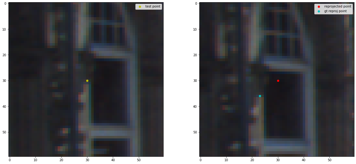
Image above illustrate how a single pixel point get reprojected from one frame to another, left image is the host frame and the right image is the target frame. The depth and camera poses estimated from MonoDepth2 are very close to the ground truth which project the point to a location near to the ground truth point, our mission is to adjust the depth to make this reprojection as close to the ground truth point as possible. Since our variable is just depth, thus we can treat this problem as a constraint optimization problem, where the constraint variable is our pose.

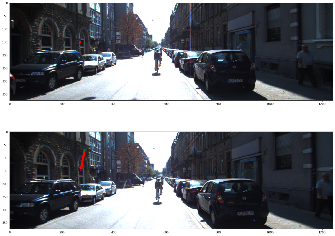
By adjust the depth, our reprojection will be moving along the tangent line bewteen the epipolar plane and image plane. In the image above, green dot depth is 4m and blue dot depth is 15m, and the maximum depth is 40m. So as you can see, the bigger depth can’t change much in the pixel coordinates, and will eventually converge into the point close to the ground truth, this constraint shares a very good property for the optimizer, since it cut the 2D local manifold into a strong convex line that further reduce the computation complexity.

From DSO (2.2 Model Formulation, page 4)

evaluating the SSD over such a small neighborhood of pixels is similar to adding first- and second-order irradiance derivative constancy terms (in addition to irradiance constancy) for the central pixel.

Same Paragraph as the above quote. They claim that the 8 pixels pattern is robust to motion blur:

Our experiments have shown that 8 pixels, arranged in a slightly spread pattern give a good trade-off between computations required for evaluation, robustness to motion blur, and providing sufficient information.

Indeed, their residual pattern works fairly well for the harsh videos, we can observe the results in the following video:

And we have tested the residual pattern in our module for a small patch (15x15). Note that DSO’s pattern strategy choose 8 pattern for their Intel SSE accumulator are only able to hold 8 threads, thus they killed one point on the right bottom corner. In our experiments, we fill that in since we are doing all these in GPU.

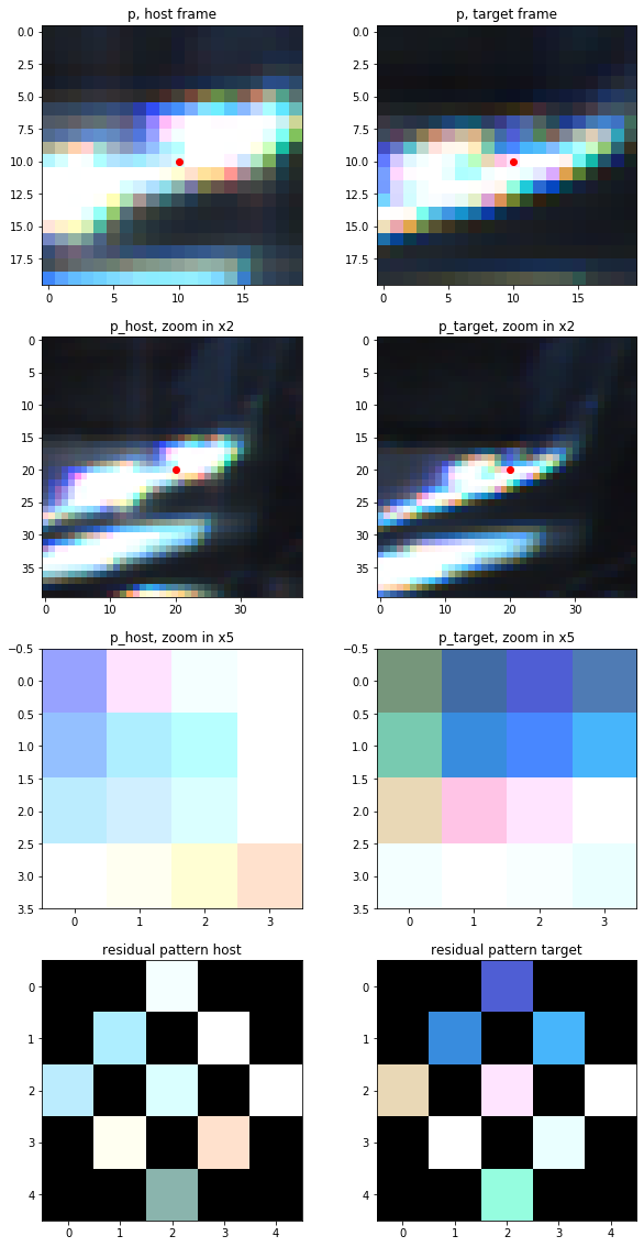
The image above shows how the residual pattern works on the ground truth reprojected point, you can see even though the point is perfectly aligned, the local region still exist some noise due to the surface reflection and occlusions, this will introduce extra error into the loss manifold and slowly corrupt the system, in the paper of DSO, the author use the huber weight to normalize the error:

Here \(\parallel \cdot \parallel_r\) is the huber weights, implementation in DSO is as following:

float residual = hitColor[0] - r2new_aff[0] * rlR - r2new_aff[1];
// huber weight of residual. -> inverse propotional to residual if above threshold.
float hw = fabs(residual) < setting_huberTH ? 1 : setting_huberTH / fabs(residual); // hw is always 0-1
// energy is the huber normalized residual.
energy += hw * residual * residual * (2 - hw);

Here the residual is single pixel’s intensity error after exposure affine correction, the r2new_aff[0] is thus \(\frac{t_je^{a_j}}{t_ie^{a_i}}\) and r2new_aff[1] is \(b_i - b_j\). The affine variables \(a_i\), \(a_j\), \(b_i\), \(b_i\) are jointly optimized in the estimation of the camera pose step. That’s why the DSO’s hessian block is 8x8, since they have 8 dimensional residuals, 6 DoF pose plus 2 affine models (8x(6+2)).

Let’s go back to our first image, where point in the frames with stable illumination to test how DSO’s photometric error works. We took the reprojected point, and calculate the photometric error along it’s neighbourhood (50x50 and 15x15).

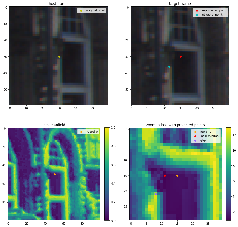
Here reproj_p is the reprojected point in the target frame with the initial estimated depth and pose, gt_p is the ground truth point corresponding to the orignal point in the host frame. From the image above, we can see that the error manifold is never convex even in the small patch (15x15) neighbourhood. Since the pattern size is pretty small, thus this error is qeuivalent to reduced mean convolve of the 3x3 kernel with the whole image. That’s why you can still see the rough shape of the original image.

Since DSO is using Gauss-Newton method to do bundle adjustment, thus they also requires the good initialization and locally convex of photometric error, thus they select the points with the higher gradient points as candidates, since the high gradient points neighbourhood will create unique combination of pattern which limited the manifold from decaying their convexity. However, in our method, we are planning to do dense depth estimation, this simple pattern strategy won’t hold our locally convex assumption, since there must be repeated textures or low texture patterns.

One of our strategy is to leverage those fixed map point as extra constrains on the optimization of the rest points, by doing this, we are assuming all points are not independently hold their own inverse depths, instead, their inverse depths should be a likelihood that are defined by it’s neighbourhood, we can thus propagate our likelihood from the known map points to those unknow points with the update of new observations (constrains). However, this method requires updating the dense map with many iterations until depth convergence, which is super computation expensive.

Thus we propose a more robust and simple method to capture the photometric error efficiently yet still keep the local convexity: random dynamic pattern.

random_pattern = gradius*np.random.rand(gsamples, 2) - gradius/2

Here the gradius, gsamples variables are inverse propotional to the local gradient score.

Here \(p_g\) is the local gradient score in point p.

\(g_r = \frac{\eta}{p_g}\) is the gradius, and \(\eta\) is the normalize constant. Same equation for the gsamples with different sample size normalizer.

The effect of the random pattern in the same reprojected point pairs is shown in the following figure:

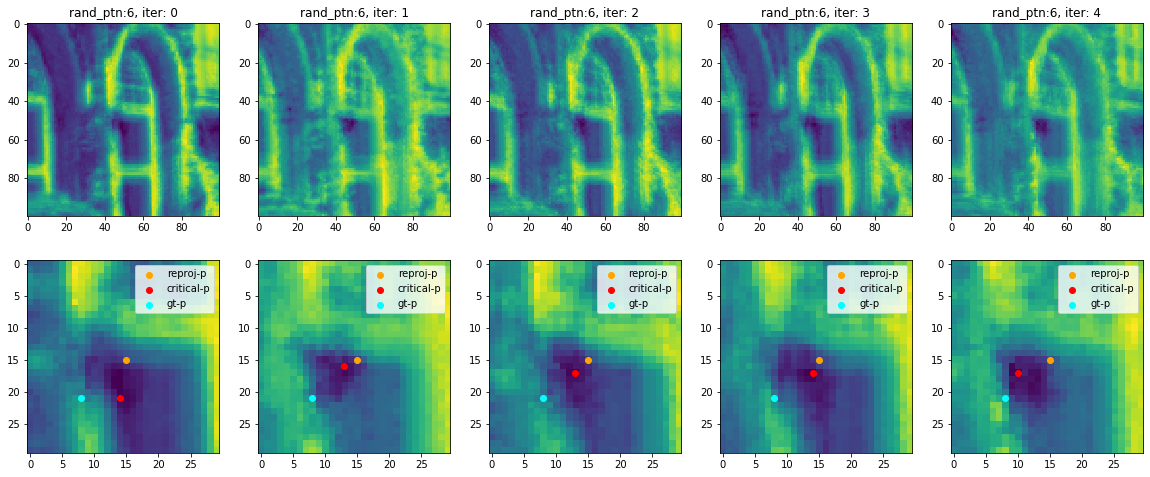
From the image above we can see that this random pattern is creating a stable local convex manifold, strict mathematic prove will be released in the upcoming publications, from this we can see that this method is equivalent to find the corners as discriptions as in feature based methods, future extensions will include the rotation invariant and scale invariant pattern. Implementation will simple be propose multiple scale or oriented patterns, but only take the smallest error as the final photometric error.

We only visualized five runs of same random sample radius size, from the figure above, we can see that this manifold is still not smooth enough nor convex. Note that when random sample radius size is small as 3, the error manifold is no difference with the DSO’s residual pattern, that is the point distribution will cover most of the pattern in the 8 point pattern.

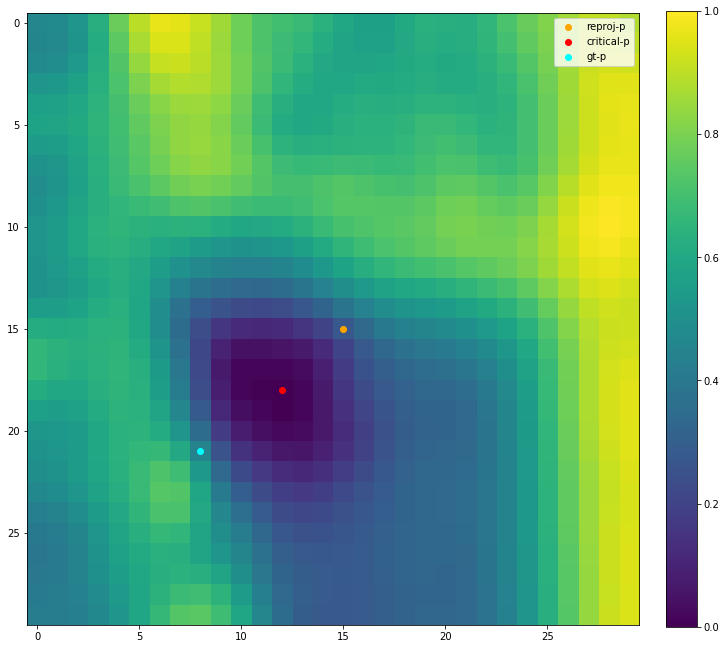
However, if we change the radius of random pattern, the error manifold will have drastic changes on the local convexity:

This figure shows that with the increased size of random sample pattern, the error is not getting more and more convex, rather this convexity is decreased and then increased, and eventually, as the sample radius increase, corrupt (become noisy), and contribute no effect on bundle adjustment optimization.

We can see that in this local region, the best random pattern size is 6, with enough convexity yet still keep the stability.

One key question is how do you evaluate the convexity?

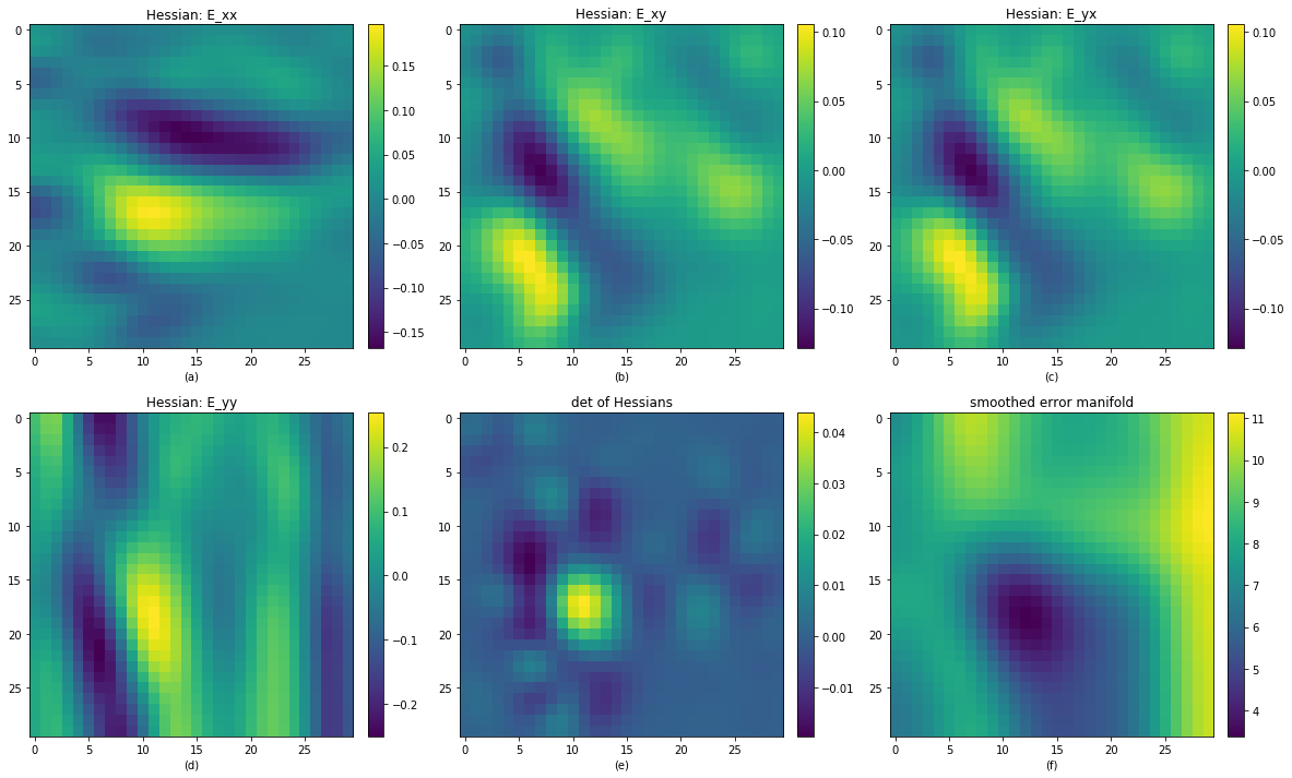
Nice question! We do it by calculate hessian of the manifold, and do distance voting:

Since our patch is centered by the reprojected point, so our distance to the reprojected point is a key concept to constrain the convex manifold to closer to our initial optimization point. By doing this, we can make sure that the error will go monotune while it’s adjusted along the epipolar line.

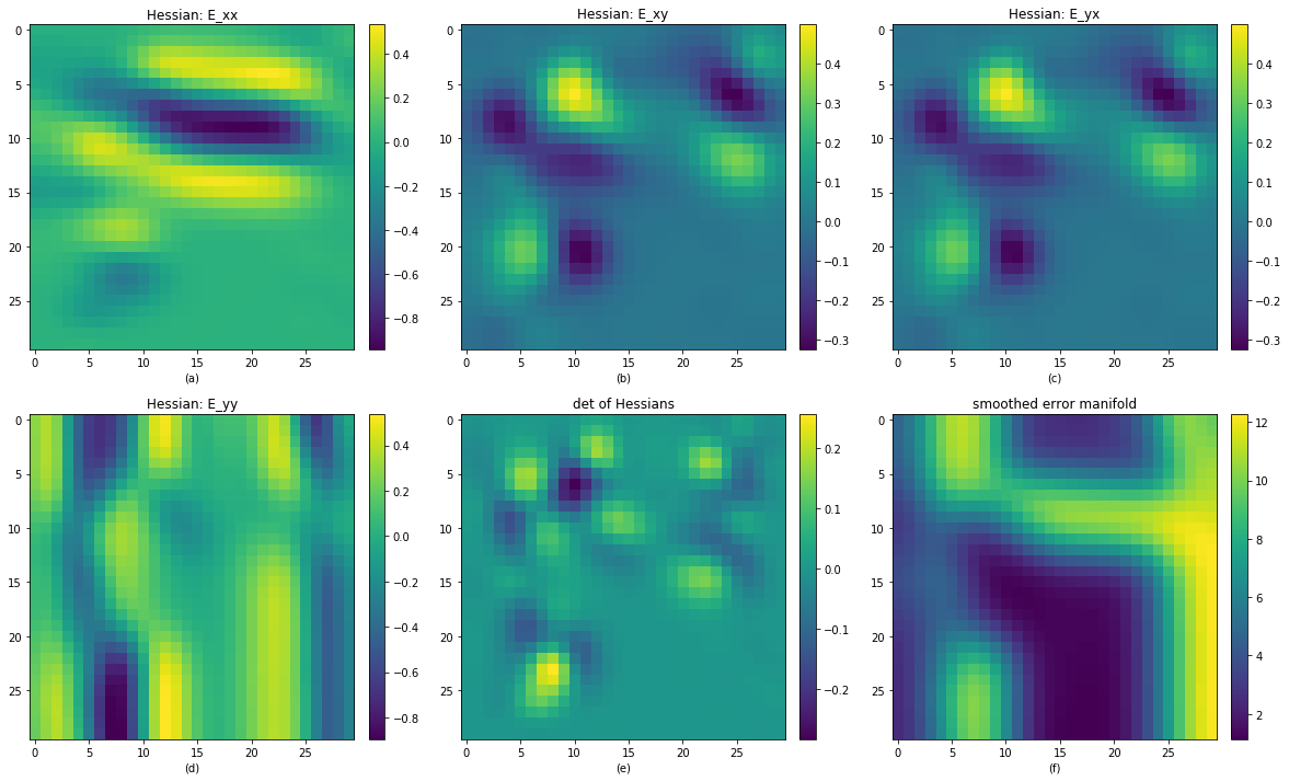
Note that we calcualte the hessian of error image, to avoid the numerical error, we have to smooth the error manifold:

Actualy we can directly use the determinant of hessian matrix in each pixel to see if this local region is convex, simply check if they are greater than zero, to see if the error hessian is positive definite, then we can say this plane is convex or not.

This is the hessian map of random pattern with radius size 6.

This is the hessian map of DSO’s residual pattern.

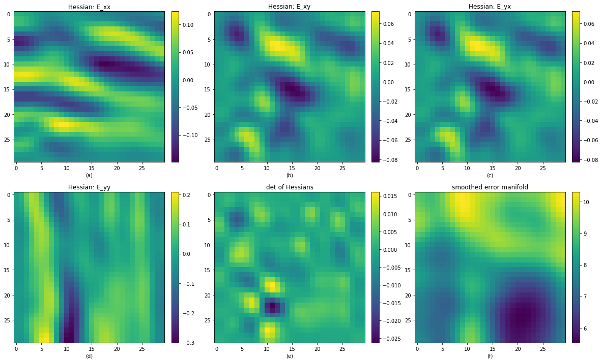
This is the hessian map of random pattern with radius size 10.

A more qualitative comparison is as following:

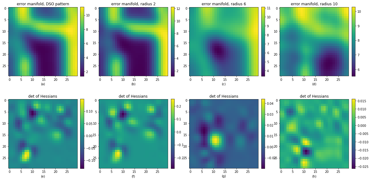
From the above image we can see that the DSO’s residual pattern is equavilant to the smaller random pattern. But none of the smaller pattern nor the larger pattern create a convex local region close to the reprojected point. Thus the dynamic random pattern can create a more robust and fast convergence rate photometric loss.