In last post, I’ve started the trial of solving the Bundle Adjustment problem with PyTorch, since PyTorch’s dynamic computation graph and customizable gradient function are very suitable to this large optimization problem, we can easily encode this problem into a learning framework and further push the optimization results into updating the depth estimations and pose estimations in a unsupervised fashion, the true beauty of this method is it introduced more elegant mathemtics to constrain the dimensionality of manifold compared to the direct photometric warping on the whole image. Plus, the sparse structure are extremely fast even apply on cpu with limited hardware (testing on nvidia tx2, cpu only).

Since we have solved pose in last post, now, we’re focusing on updating the depth for each active point hessian. And before we start, let’s see how this pipeline works:

Assume we know the pose already (solved by last post), and we have a very noisy initial of depth from monodepth2, then let’s reproject a point from host frame into target frame:

Here \(p\) is the point in host frame, \(p'\) is the point in target frame, both are in pixel coordinates, and \(K\) is intrinsic, \(T_i\) is host to target 3x4 traformation matrix which can be expreseed in SE3, a 1x6 vector. \(d\) is the depth of point \(p\), we put it outside \(p\) since we are going to apply it’s depth after it’s recovery into world coordinate.

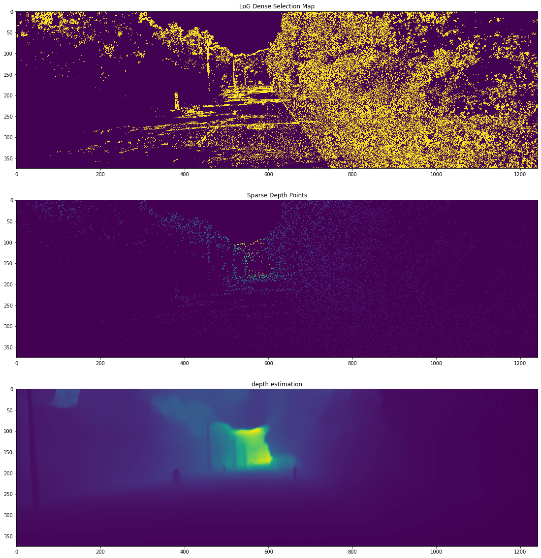
Since our depth estimation is off, so the projection will be slightly off too, results on kitti will be like this:

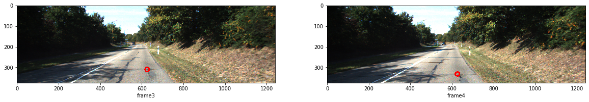
Let’s zoom in:

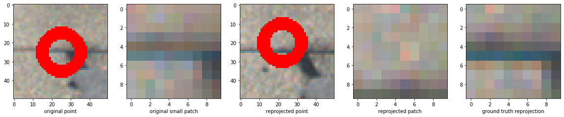
Now you can see that this reprojection is kind of 6 pixels below the groud truth. I manually piecked a higher gradient area for illustration, however, there are large portion of low gradient regions, for those part of image, we can use the nearby boundary to approximate that area as a local plane and recover depth use this plane.

we are solving this depth by find the gradient of it w.r.t the reprojection error, namely, photometric error.

let’s expand this further more:

and continue to expand:

Now this equation will be very long that’s bad for display (you can derive this equation from matlab anyway), let’s consider backward:

to be more clear the chain should look like this:

Okay, that’s simple right? current depth of p is mostly propotational to the product of error and local gradient and the last guess depth of p.

Now, let’s focus on the easiest part, solving depth from the selected point hessians (with high local gradient), the PyTorch implementation is easy, since autograd function will take care most part of the gradient, the only thing we need to care for is to implement the backward gradient function of \(I(p)\):

Let’s first define the point and camera intrinsic tensor:

device = torch.device("cuda:0")
p = torch.tensor([x_, y_, z_], dtype=torch.double, requires_grad=True)
p = torch.reshape(p, (3, 1))
K = torch.tensor(data.calib.K_cam3, dtype=torch.double)

Then get the image tensor and image gradient (gradient function was in my deep vo repo, too length to post here):

data_img_current = torch.tensor(np.array(data.get_cam3(img_id)))
data_img_next = torch.tensor(np.array(data.get_cam3(img_id+1)))
# gradient of image
img_cur_dx_, img_cur_dy_ = image_gradients(data_img_current)
img_next_dx_, img_next_dy_ = image_gradients(data_img_next)
# convert those things to tensors
img_cur_dx = torch.tensor(img_cur_dx_, dtype=torch.double)
img_cur_dy = torch.tensor(img_cur_dy_, dtype=torch.double)
img_next_dx = torch.tensor(img_next_dx_, dtype=torch.double)
img_next_dy = torch.tensor(img_next_dy_, dtype=torch.double)

Followed with the tranformation matrix \(T_{h2t}\), from host to target:

T = torch.tensor(np.dot(pose_next, np.linalg.inv(pose_current)))

And we can now apply the reprojection safely:

pki = torch.mm(K.inverse(), p)
ext_homo = torch.ones(1,1).double()
pki = torch.cat((pki, ext_homo), dim=0)
pTki = torch.mm(torch.tensor(np.linalg.inv(pose_current)), pki)
pTki = torch.mm(torch.tensor(pose_current), pTki)
pkTki = torch.mm(K, pTki[0:3])

Now we get the coordinate of the reprojected point (experimental results):

tensor([[ 8.0176],
        [15.0874],
        [ 1.0000]], dtype=torch.float64, grad_fn=<DivBackward0>)

Since PyTorch didn’t define this gradient of image per pixel, we have to make our own:

class photometric_error(torch.autograd.Function):
    @staticmethod
    def forward(ctx, input):
        # input: px py, p'_x, p'_y which is coordinate of point in host frame, and point in target frame
        # forward goes with the image error compute
        ctx.save_for_backward(input)
        return data_img_next[input[0].long(), input[1].long()]
    @staticmethod
    def backward(ctx, grad_output):
        input, = ctx.saved_tensors
        grad_input = grad_output.clone()
        grad_input = grad_input.double()
        pnext_dx = img_next_dx[input[0].long(), input[1].long()].clone().double()
        pnext_dy = img_next_dy[input[0].long(), input[1].long()].clone().double()
        print(pnext_dx)
        grad_dx = grad_input*pnext_dx
        grad_dy = grad_input*pnext_dy
        grad_ret = grad_dx + grad_dy
        grad_ret = torch.reshape(grad_ret, (3, 1))
        print(grad_ret)
        return grad_ret

Extend the torch.autograd.Function and implement the forward, backward functions so that we get the gradient chain hooked.

Then let’s just apply this function and caculate the loss:

perr = photometric_error.apply
peP = perr(pkTki)
loss = (peP - data_img_current[x_, y_]).pow(2).sum()

and before you apply the backward pass, remind the tensors to keep their gradients:

peP.retain_grad()
pkTki.retain_grad()
p.retain_grad()

Now, you can safely apply loss.backward():

loss: tensor([2.2309], dtype=torch.float64)

Our gradient \(\frac{\partial E}{\partial I}\) is as following:

tensor([[468.0704],
        [434.6368],
        [585.0880]], dtype=torch.float64)

and let’s see the gradient of p:

tensor([[  0.184868],
        [  0.171663],
        [-4.072140]], dtype=torch.float64)

Let’s make this whole pipeline into a loop and loop until loss doesn’t change (usually 3 steps) and we can get our converged depth.

Now we can just apply CSPN or any sparse propagation method to update the depth proposals to finish our unsupervised training loop.