
Solve BA with PyTorch Optimization Backend
This post shows how to use LBFGS optimizer to solve Bundle Adjustment.

Structure from Motion and Visual SLAM applications are heavily dependent on inter-frame geometries, recent deep methods like SfMLearner, MonoDepth, DDVO and many other methods managed to isolate the joint optimization of camera pose and the estimation of depth. They treat the training of pose network as supervised learning, since most datasets offers ground truth camera pose. This trick circumvent the dense optimization problem in BA and extremely simplified the learning life cycle with back warping and direct photometric error losses. However, one can still argue that the parameter manifold of SE3 learnt from pose network can be limited and dataset dependent, see detailed explanation from here: E2E PoseNet. Besides, the pose estimations are always in limited distributions which will be very unfriendly for UAV with large maneuver degrees. To make this pipeline more robust, we introduced our proposal on extend the depth and pose estimation with a windowed Bundle Adjustment Backend.
Here’s a simple illustration on how depth and pose network works:

Unlike the traditional depth and pose estimation system which treat pose and depth estimation separately (SfMLearner, MonoDepth2, BANet) we are going to jointly optimize pose \(\xi\) and dense depth map \(d_i\) for each BA iteration, from the diagram above you can see we just applied two iterations of dense BA since we are going to make sure this whole pipeline goes real time, even with the help of GPU.
Inspired by DSO, our pipeline is also using coarse to fine fashion. The reason is: pose of consequtive frames captured at normal frequency are normally small enough, thus can be estimated by coarse and small scale of image, with this coarse pose, we are able to refine our initial depth map guess quickly, and then propagate this refined depth map into larger scale space. By this way, we can quickly initialize the depth and pose with a reasonable prior, and use this initial state to optimize will reach a good critical point which has higher change to be global minimum (depth recovering is an ill-pose problem since image manifold is super non-convex, that’s why we need a good initialization). Now after convergence of the dense depth map, we will inturn adjust pose again (that’s why they call Bundle Adjustment, they are adjusting two end of the bundle projection ray: camera end \(\xi\), and world end \(d\)). Eventually, we will use them to do backwarping and calculate the photometric loss, smoothness loss, occlusion loss and affine loss.
Now with knowing enough big picture on what we should do, let’s take a close look on how to implement them. First step is to estimate pose, which was introduced in my last post. Then we can do depth estimation with the following equation:
\[h(I_{t'}, \xi_1, d_2) = I_{t'}[KT_{w2c}\xi_1T_{w2c}^{-1}d_{2, i}[p_i]K^{-1}p_i] \forall i \in \theta\]Here \(\xi\) is the camera pose and the \(\theta\) is the selected gradient point sets.
Let’s take any sample point from selected points in my previous post: gradient based pixel selector
v_ = chosen_p[0]
u_ = chosen_p[1]
z_ = visualizer_map[v_, u_]*10
d = torch.autograd.Variable(torch.tensor([z_], dtype=torch.double)).requires_grad_()
Here we use autograd.Variable to define our point since we are going to optimize it out later on in LBFGS loop. Note that you need to apply requires_grad_() function in the end since we need this variable in the leaf node of the computation graph, otherwise optimizer won’t recognize it.
Since we only care about the depth, so we isolated the point and the depth variable:
pxyz = torch.tensor([u_, v_, 1]).double()
pxyz tensor’s z value is set as 1. We are going to recover the depth later on.
tensor([[725.],
        [135.],
        [  1.]], dtype=torch.float64)
Since the only thing we need to estimate is depth, thus u_ and v_ are regarded as constants for each point in the depth map. We extend the depth into 3D point w.r.t to current camera coordinate, and then apply the inverse intrinsic to project into world coordinate.
pki = torch.mm(K.inverse(), p)
pki = d*pki
tensor([[ 4.7520],
        [-1.5582],
        [29.7016]], dtype=torch.float64, grad_fn=<MulBackward0>)
Here’s \(K\) and \(T_{w2c}\):
K:
tensor([[721.5377,   0.0000, 609.5593],
        [  0.0000, 721.5377, 172.8540],
        [  0.0000,   0.0000,   1.0000]], dtype=torch.float64)

T_w2c = torch.tensor(t_imu2cam, dtype=torch.double)

T_w2c:
tensor([[ 9.9875e-04, -9.9999e-01,  4.2594e-03, -7.8463e-01],
        [ 8.4169e-03, -4.2508e-03, -9.9996e-01,  7.1945e-01],
        [ 9.9996e-01,  1.0346e-03,  8.4126e-03, -1.0891e+00],
        [ 0.0000e+00,  0.0000e+00,  0.0000e+00,  1.0000e+00]],
       dtype=torch.float64)

T_w2c.inverse():
tensor([[ 9.9875e-04,  8.4169e-03,  9.9996e-01,  1.0838e+00],
        [-9.9999e-01, -4.2508e-03,  1.0346e-03, -7.8044e-01],
        [ 4.2594e-03, -9.9996e-01,  8.4126e-03,  7.3192e-01],
        [ 0.0000e+00,  0.0000e+00,  0.0000e+00,  1.0000e+00]],
       dtype=torch.float64)
With all those known parameters defined, we can now apply the reprojection:
# extend the point to homogeneous coordinate
ext_homo = torch.ones(1,1).double()
pki = torch.cat((pki, ext_homo), dim=0)
-------------------------------------------------------------
output:
tensor([[ 4.7520],
        [-1.5582],
        [29.7016],
        [ 1.0000]], dtype=torch.float64, grad_fn=<CatBackward>)
-------------------------------------------------------------
pTwcki = torch.mm(T_w2c.inverse(), pki)
pTwcki
-------------------------------------------------------------
output:
tensor([[30.7759],
        [-5.4951],
        [ 2.5602],
        [ 1.0000]], dtype=torch.float64, grad_fn=<MmBackward>)
-------------------------------------------------------------
pTTwcki = torch.mm(torch.tensor(pose_current), pTwcki)
pTTwcki = torch.mm(torch.tensor(np.linalg.inv(pose_next)), pTTwcki)
pTTwcki
-------------------------------------------------------------
output:
tensor([[29.3777],
        [-5.4914],
        [ 2.5796],
        [ 1.0000]], dtype=torch.float64, grad_fn=<MmBackward>)
-------------------------------------------------------------
pTTTki = torch.mm(T_w2c, pTTwcki)
pTTTki
-------------------------------------------------------------
output:
tensor([[ 4.7471],
        [-1.5895],
        [28.3036],
        [ 1.0000]], dtype=torch.float64, grad_fn=<MmBackward>)
-------------------------------------------------------------
pKTTTki = torch.mm(K, pTTTki[0:3])
pKTTTki
-------------------------------------------------------------
output:
tensor([[20677.8739],
        [ 3745.5288],
        [   28.3036]], dtype=torch.float64, grad_fn=<MmBackward>)
-------------------------------------------------------------
pKTTTki = pKTTTki/pKTTTki[-1]
-------------------------------------------------------------
output:
tensor([[730.5752],
        [132.3342],
        [  1.0000]], dtype=torch.float64, grad_fn=<DivBackward0>)
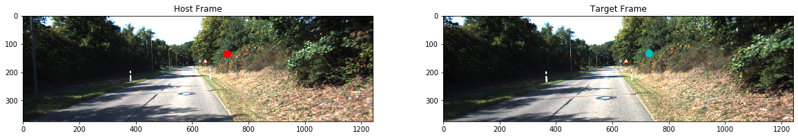
Here pKTTTki is reprojected into the camera coordinate in the target frame:
tensor([[730.5752],
        [132.3342],
        [  1.0000]], dtype=torch.float64, grad_fn=<DivBackward0>)
Compared to the original coordinate from host frame:
tensor([[725.],
        [135.],
        [  1.]], dtype=torch.float64)
Let’s plot them to check whether this align or not:
Notice that we keep out gradient function hooked in each step, so that the backward on loss will eventually navigate us to the exact gradient we want.
Before calculate our photometric loss, let’s define our own computation graph for the image gradients, this function helps us to hook up the photometric error with the previous projection gradients and connect the computation graph all the way back to our required gradient: d.grad.
class img_grad(torch.autograd.Function):
    @staticmethod
    def forward(ctx, input):
        # input: px py, p'_x, p'_y which is coordinate of point in host frame, and point in target frame
        # forward goes with the image error compute
        ctx.save_for_backward(input)
        return data_img_next[input[1].long(), input[0].long()].double()
    @staticmethod
    def backward(ctx, grad_output):
        input, = ctx.saved_tensors
        grad_input = grad_output.clone()
        grad_input = grad_input.double()
        pnext_dx = img_next_dx[input[1].long(), input[0].long()].clone().double()
        pnext_dy = img_next_dy[input[1].long(), input[0].long()].clone().double()
        grad_dx = grad_input*pnext_dx
        grad_dy = grad_input*pnext_dy
        damping_lambda = 1 # 0.001
        grad_ret = damping_lambda *(grad_dx + grad_dy)
        grad_ret = torch.reshape(grad_ret, (3, 1))
        return grad_ret
Here img_next_dx, img_next_dy are image gradient on x direction and y direction, see my repo for detailed function, since they are too lengthy.
Now we need to apply this function, this apply is simply return the function reference to imgrad so that you can call imgrad directly later on, it will return the image pixel value, and propogate the gradient from loss back to the point pKTTTki and then all the way back to d.
imgrad = img_grad.apply
peP = imgrad(pKTTTki)
-------------------------------------------------------------
output:
tensor([[50., 80., 84.]], dtype=torch.float64,
       grad_fn=<photometric_errorBackward>)
And we compute the loss with the simple MSE for each channel, this is super problematic, we can see the results on the later on optimization stage.
loss = (peP2 - data_img_current[v_, u_].double()).pow(2).sum().double()
-------------------------------------------------------------
output:
tensor(7957., dtype=torch.float64, grad_fn=<SumBackward0>)

d.grad:
tensor([0.0023], dtype=torch.float64)
Yes, you can see this gradient is small enough, that means we are already having a very good estimation. But if you throw the above steps into optimizer like LBFGS, it will hit out of the pot and stuck at a high ridge:
opt = torch.optim.LBFGS([d],lr=0.1)
for i in range(10):
    def closure():
        opt.zero_grad()
        pxyz = torch.tensor([u_, v_, 1]).double()
        p2 = torch.reshape(pxyz, (3, 1)).double()
        K = torch.tensor(data.calib.K_cam3, dtype=torch.double)
        T_w2c = torch.tensor(t_imu2cam, dtype=torch.double)
        T = torch.tensor(np.dot(pose_next, np.linalg.inv(pose_current)))
        p2 = torch.mm(K.inverse(), p2)
        p2 = d * p2
        ext_homo = torch.ones(1,1).double()
        p2 = torch.cat((p2, ext_homo), dim=0)
        p2 = torch.mm(T_w2c.inverse(), p2)
        p2 = torch.mm(torch.tensor(pose_current), p2)
        p2 = torch.mm(torch.tensor(np.linalg.inv(pose_next)), p2)
        p2 = torch.mm(T_w2c, p2)
        p2 = torch.mm(K, p2[0:3])
        p2 = p2/p2[-1]
        d.requires_grad_()
        peP2 = perr(p2)
        loss = (peP2 - data_img_current[v_, u_].double()).pow(2).sum().double()
        loss.backward(retain_graph=True)
        print("p2: {}".format(p2.data))
        print("d: {}".format(d.data))
        print("loss: {}".format(loss.data))
        return loss
    opt.step(closure)
Here’s the outputs:
-------------iter: 0-----------------
p2: tensor([[730.8892],
        [132.2287],
        [  1.0000]], dtype=torch.float64)
d: tensor([28.0992], dtype=torch.float64)
loss: 7957.0
-------------iter: 0-----------------
p2: tensor([[730.9101],
        [132.2217],
        [  1.0000]], dtype=torch.float64)
d: tensor([27.9992], dtype=torch.float64)
loss: 7957.0
-------------iter: 1-----------------
p2: tensor([[730.9101],
        [132.2217],
        [  1.0000]], dtype=torch.float64)
d: tensor([27.9992], dtype=torch.float64)
loss: 7957.0
-------------iter: 1-----------------
p2: tensor([[731.3318],
        [132.0799],
        [  1.0000]], dtype=torch.float64)
d: tensor([26.1257], dtype=torch.float64)
loss: 1194.0
-------------iter: 1-----------------
p2: tensor([[731.2893],
        [132.0942],
        [  1.0000]], dtype=torch.float64)
d: tensor([26.3026], dtype=torch.float64)
loss: 1194.0
-------------iter: 2-----------------
p2: tensor([[731.2893],
        [132.0942],
        [  1.0000]], dtype=torch.float64)
d: tensor([26.3026], dtype=torch.float64)
loss: 1194.0
-------------iter: 2-----------------
p2: tensor([[731.0090],
        [132.1884],
        [  1.0000]], dtype=torch.float64)
d: tensor([27.5348], dtype=torch.float64)
loss: 1194.0
-------------iter: 3-----------------
p2: tensor([[731.0090],
        [132.1884],
        [  1.0000]], dtype=torch.float64)
d: tensor([27.5348], dtype=torch.float64)
loss: 1194.0
-------------iter: 3-----------------
p2: tensor([[730.7572],
        [132.2730],
        [  1.0000]], dtype=torch.float64)
d: tensor([28.7501], dtype=torch.float64)
loss: 7957.0
-------------iter: 3-----------------
p2: tensor([[730.7587],
        [132.2726],
        [  1.0000]], dtype=torch.float64)
d: tensor([28.7429], dtype=torch.float64)
loss: 7957.0
-------------iter: 4-----------------
p2: tensor([[730.7587],
        [132.2726],
        [  1.0000]], dtype=torch.float64)
d: tensor([28.7429], dtype=torch.float64)
loss: 7957.0
-------------iter: 4-----------------
p2: tensor([[730.7601],
        [132.2721],
        [  1.0000]], dtype=torch.float64)
d: tensor([28.7358], dtype=torch.float64)
loss: 7957.0
Yes, you can see the optimizer found the global optimal at 3rd iteration:
-------------iter: 3-----------------
p2: tensor([[731.0090],
        [132.1884],
        [  1.0000]], dtype=torch.float64)
d: tensor([27.5348], dtype=torch.float64)
loss: 1194.0
but quickly overshoot into another direction that has even higher loss than the original reprojection. The reason this happens is in two fold:
- L-BFGS algorithm will not converge in the true global minimum even if the learning rate is very small.
- Discretized image space makes the optimization pretty hard since the squared error loss function in single pixel is not smooth at all, let alone the convexity.
“Notice that L-BFGS and other Quasi-Newton algorithms require at least local convexity.” Not true. SR1 Quasi-Newton (including L-SR1 and L-SR1-B) may be able to handle indefinite or even concave objective functions, even near or at the optimum, at least if used within a trust region framework.
Yes, one remedy could be introduce the trust region framework and offer the optimizer a damping factor. Yet this still can’t solve the non-convex property on the image side.
That’s why DSO introduced a residual pattern which combines the nearby points as comparisons to smooth out the loss manifold. However this is still problemtic, since this manifold will eventually hit into a flat plane when the point is in repeated texture local region, how to solve that? Well, one way we can try is still pyramid method, hoping in another scale space we can hit into boundary of the local region and remove the nullspace, another way is to introduce deep methods to solve this problem, by converting the points into feature maps, n points with n feature maps and we compare the feature maps’ distance to construct a very smooth loss function which is more friendly on second order optimizers.
By simply apply the 9 dimensional residual pattern and get them reproject into the target frame, we can get the simple SSD loss heat map as following:
Seems like a convex platform hey? How about the following map, this is the loss manifold on the enlarged trust region, you can find out how non-convex this map is:
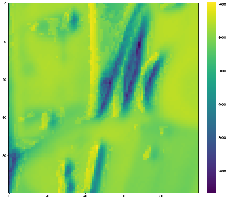
That’s exactly why DSO and any direct methods requires a very good initialization, since the optimization backend needs a really convex setting, especially for the second order non-linear ones.