Since Bundle Adjustment is heavily depending on optimization backend, due to the large scale of Hessian matrix, solving Gauss-Newton directly is extremely challenging, especially when solving Hessian matrix and it’s inverse. Scale of Hessian matrix is depending on number of map points, so to this end, we can first estimate the point inverse depths and then update the poses in two stage manner, however, this requires a very good initializaiton for depth estimation, and requires a convex local photometric loss to make sure positive definite property of the Hessian.

Figure above illustrated Gauss-Newton method pipeline, which is iteratively estimating \(\Delta x\) and updating \(x\) to the convergence point where \(\Delta x\) close to zero. This pipeline can be well modeled by PyTorch where we can easily use autograd to solve Jacobians and pseudo-inverse of Hessian matrix.

Here we are regarding the big Hessian matrix as a layered weights, each row of Hessian matrix is a layer of MLP, and the gradients propapated backwards is exactly the update of camera pose, after several trials, we can use this MLP to capture the transformation \(\Delta x\) in between each frame.

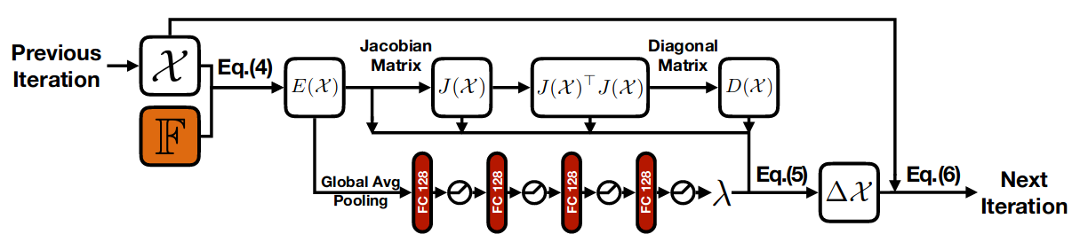
Figure above is copyright of BANet

Similarly BANet has done the same job using the MLP to learn the damping factor \(\lambda\) which is mimic the LM method to normalize the searching trust region. And convert this iterative pipeline into a recurrent structure.

# two frames:
hostFrame = frame_window[0]
targetFrame = frame_window[-1]
# define the H matrix
H_old = torch.randn(M, N)
b_old = torch.randn(N, 1)
# reshape input H matrix:
x = torch.randn(N, 1, requires_grad=True)
# initial learning rate
lr = 1e-5
optimizer = optim.LBFGS([x], lr=lr)
def closure():
    H_new, b_new, loss = calcResAndGS(x)
    H_old = H_new
    b_old = b_new
    optimizer.zero_grad()
    loss.backward()
    return loss
for lr in lr * .5**np.arange(10):
    optimizer.step(closure)

Here function calcResAndGs is the major function to calculate loss and estimate Hessian and Jacobian matrix from current pose:

def calcResAndGS(x):
    JbBuffer = torch.zeros([x.shape[0], npts], dtype=torch.float32)
    inc = np.linalg.inv(H_old[:6, :6]) * b_old
    refToNew = inc * sophus.SE3(x)
    # loop all selected points
    e = torch.zeros([npts], dtype=torch.float32)
    for i in range(npts):
        reproj_p = torch.matmul(refToNew, point[i])
        idepth = reprj_p[-1]
        reproj_p = torch.matmul(K, reproj_p)
        pe = targetFrame[reproj_p[0], reproj_p[1]] - hostFrame[point[i][0], point[i][1]]
        e[i] = pe
        dIdx = targetFrame.dx[reproj_p[0], reproj_p[1]]
        dIdy = targetFrame.dy[reproj_p[0], reproj_p[1]]
        u = reproj_p[0]
        v = reproj_p[1]
        # dedxi -> partial to the camera pose
        jbBuffer[0, i] = idepth * dIdx
        jbBuffer[1, i] = idepth * dIdy
        jbBuffer[2, i] = -idepth * (u * dIdx + v * dIdy)
        jbBuffer[3, i] = -u * v * dIdx - (1 + v * v) * dIdy
        jbBuffer[4, i] = (1 + u * u) * dIdx + u * v * dIdy
        jbBuffer[5, i] = -v * dIdx + u * dIdy
    H = torch.matmul(jbBuffer.T, jbBuffer)
    b = torch.matmul(jbBuffer.T, e)
    loss = torch.sum(e)
    return H, b, loss

According to perturbation lemma (BA in DSO):

Here \(\delta \xi\) is the small perturbation delta and this equation decomposed derivative of lie group into two parts: partial derivative to the 3d point and the partial derivative of the perturbation delta, since we know that:

Now the second partial is: \(\frac{\partial P'}{\partial \delta \xi} = \frac{\partial (Tp)}{\partial \delta \xi} = \begin{bmatrix} I & -P'^{\wedge} \ 0 & 0 \ \end{bmatrix}\)

Note that the matrix above is a 4x4 matrix in homogeneous coordinate, and we only extract the first 3 rows:

For simplicity, we note that \(\frac{\partial e}{\partial \xi}\) as \(F\) and \(\frac{\partial e}{\partial p}\) as \(E\).

Here the Jacobian matrix is exactly the hstack of matrix E and F. As shown in the previous code, first three entries of jbBuffer is exactly partial w.r.t rotation vector, and last 3 entries are for translation vector.

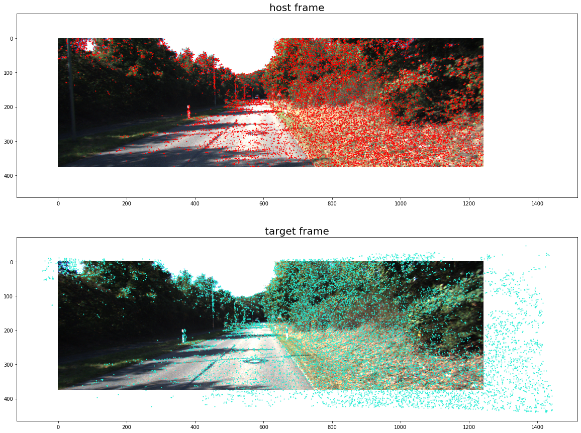
The whole pipeline converges around 10 iterations, we can then apply our converged camera pose \(\xi\), apply the reprojection to see the effect: