When I interview many people for their basic understanding of convolutional neural network, people are always simplify this into a single convolution kernel run through the sliding window. However, few of them can really recall what’s going on inside the actual machine. Here’s a tutorial to recap your crashing course again and then we will dive into the sparse convolution.

But Before starting our journey, lets have a close look at how 2D convolution at /images works, you may skip this part since its too basic.

A convolutional neural network is usually explained with the above figure. Where a RGB image is processed with a ConvNet depicted with a transposed trapezoid. Then the rgb image is transformed as a set of feature maps with smaller shape.

Then a detailed image will prompt and show that the kernel filter will slide through the origin image and output one value for that kernel which aggregate the neighborhood.

I admit that the way people illustration ConvNet is very intuitive; however, few people have tried to explore and explain what really does inside the computer.

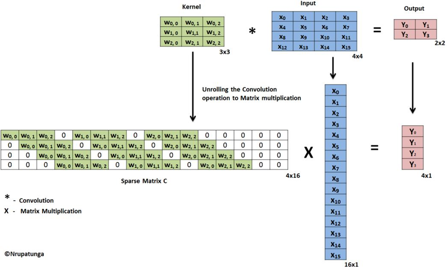
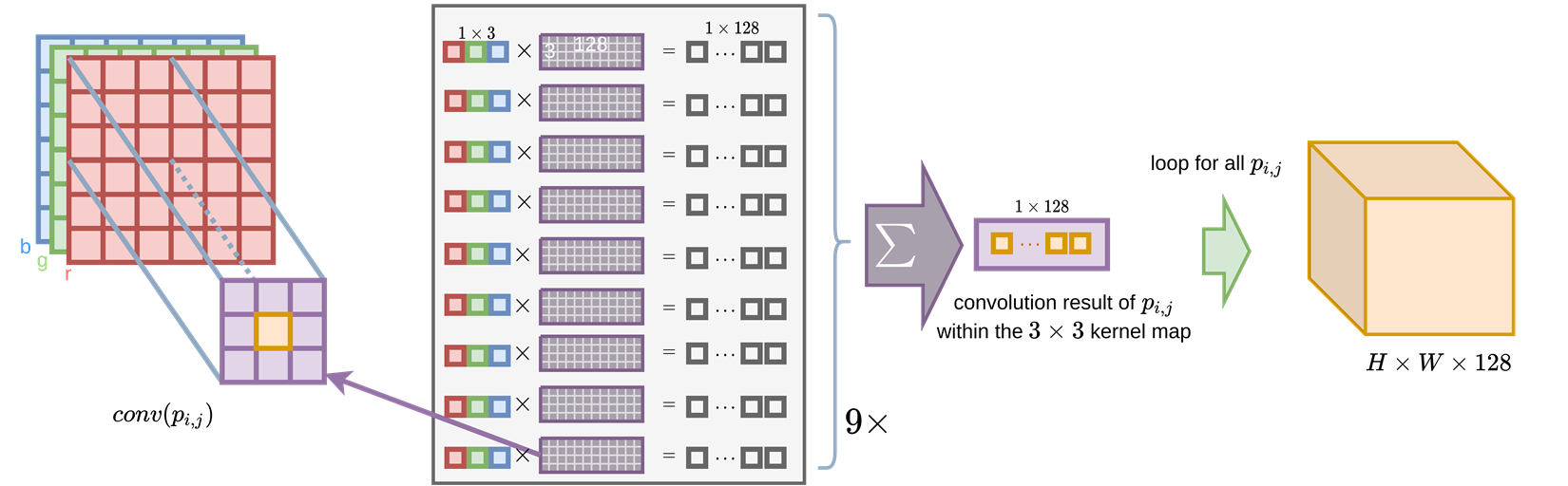
As shown above, this is a typical step what people do when we are performing a convoltion operation in computer, the weight matrix is unrolled based on the size of kernel and the size of the input size with zero padding, for a 3x3 size kernel, the first second and third row is shift repeatedly w times where w is the size of the image width. This is equivalent to do the sliding window in normal convolution.

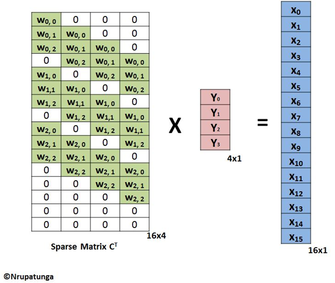
Similarly, the transpose conv which recover the image shape back to the higher resolution is just applying the multiplication of the transposed unrolled weight matrix, then the image will be recovered back to the original size, actually we can recover back to any scale by control the size of the unroll padding.

Given those background information, it’s very interesting to think about how the weight matrix is stored in the memory?

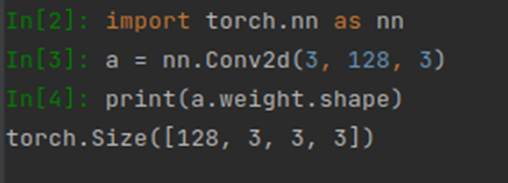
Let’s try it our by typing the following code in the editor and see how it works:

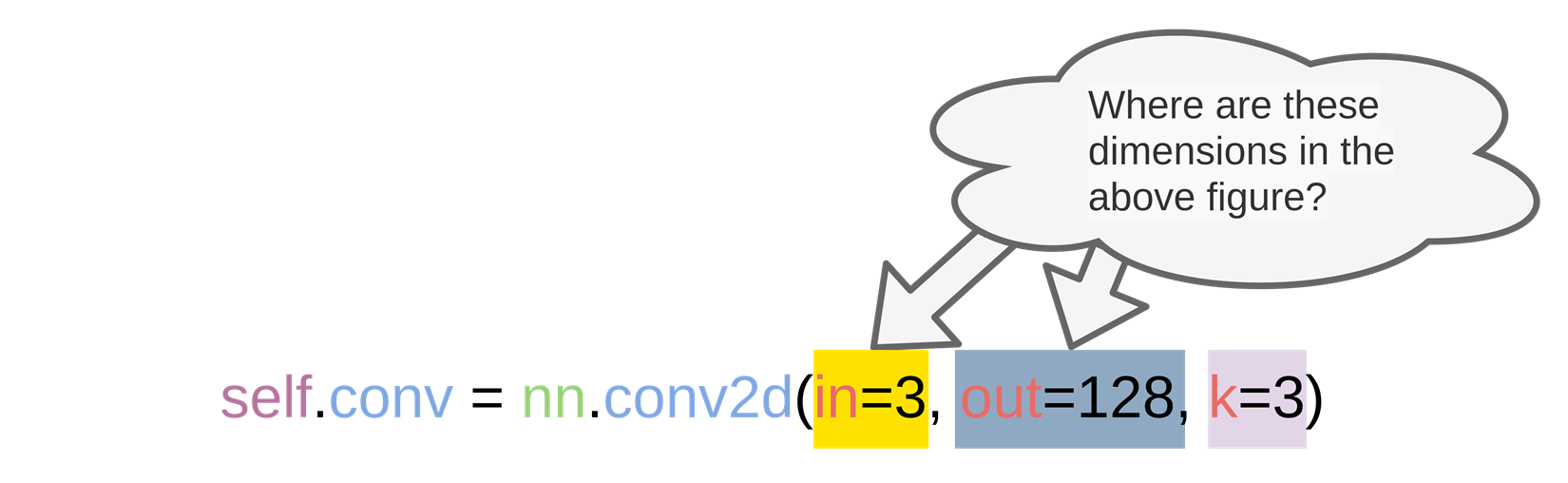
import torch.nn as nn
conv = nn.Conv2d(3,128,3)
print(a.weight.shape)

The output is:

Explain why the shape is [128, 3, 3, 3]:

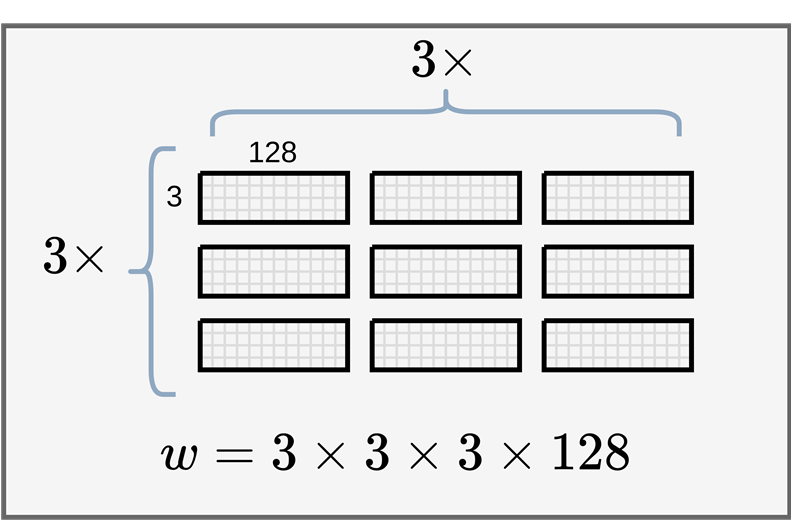
Each cell of 3X3 kernel is actually a input_channel x output_channel shaped matrix. What this matrix does is that it project the feature vector of each pixel in the original input tensor into the output channel feature vector, you can imagine it as a coordinate transformation process, we are projecting a 3D data into 128D.

As we all know that when we raising the dimension of manifold the decision boundary will be easier to be found by optimizer. That’s part of the reason why people often increase the channel size and observed the performance increase. However, just increasing the feature channel size does not guarantee the increase of performance, instead, it might cause the network to be much sparse and hard to converge. If you search the internet, there are lots of smart people working on solving this problem and try to expand the width of a network. Since it can really remember a lot of details!

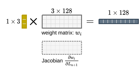
When we are training the network, the projection weight matrix for each pixel in the kernel is maintaining a shadow cache that stores the gradient matrix (jacobian matrix).

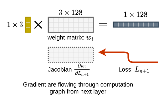
The gradients will be accumulated in the cache for all the batches that’s why when you set a higher batch size the gpu memory will grow.

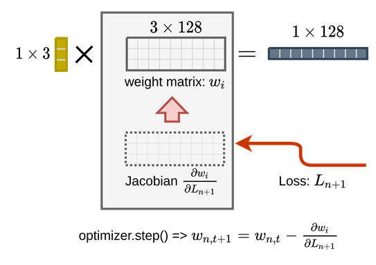
When the batch is finished the gradient will be averaged and applied back to the matrix original weight matrix in-place to update the parameter of the network.

Lets bring this detail back to the beginning, we can see that there is a better way to explain the convolution for people to really dig into the implementation side of it.

Sparse Conv

Now with enough background of ordinary convolution of a 2D image, we can think about how a convolution can generalize from it.

Where \(i\) belongs to \(N\), the kernel region offset with respect to the current position \(u\).

When we are considering the sparse data, the general formulation of convolution is very easy to be extended, just change the \(i\) as the kernel regiion where the raw data is not empty. By doing so, we do not update the pixel of the kernel filter if there is no data in the original place for a given convolution step.

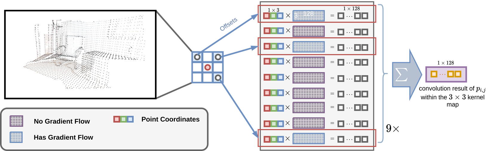
That’s it, we do not update the empty cells in sparse convolution.

And it will degenerate to point-wise mlp if the kernel region size is set as 1 or there is no neighborhood inside the current query point.

One important thing to note is that we need to cover the coordinate changes when we apply the convolution, unlike dense image, the sparse 3d point cloud have empty in most space, how to tell the down-sampled points to recover back to the original resolution is a very challenging task. Thus people are proposing the coordinate hashing to map the coordinates in different hierarchial layers of convolution and transpose convolution.

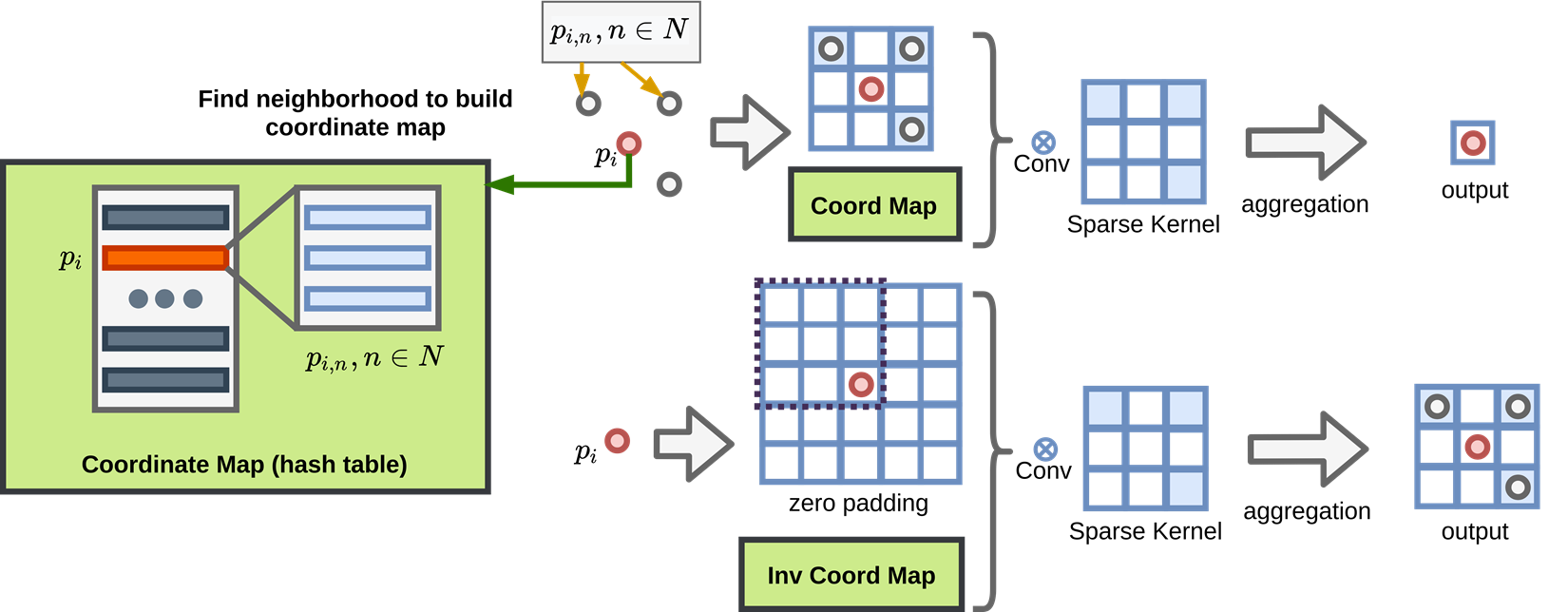
In the Figure above, the transpose conv use the convolutional coordinate hashmap recorded during the convolution process.

However, when we are trying to seek for a way to complete the voxelized tensor where there is no original coordinate hashmap generate from convolution layers, the situation changes.

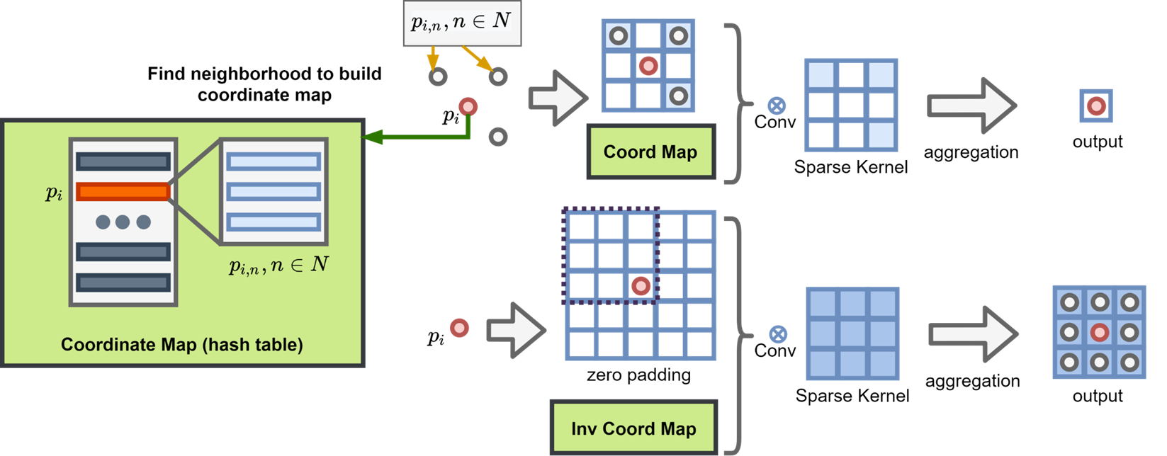
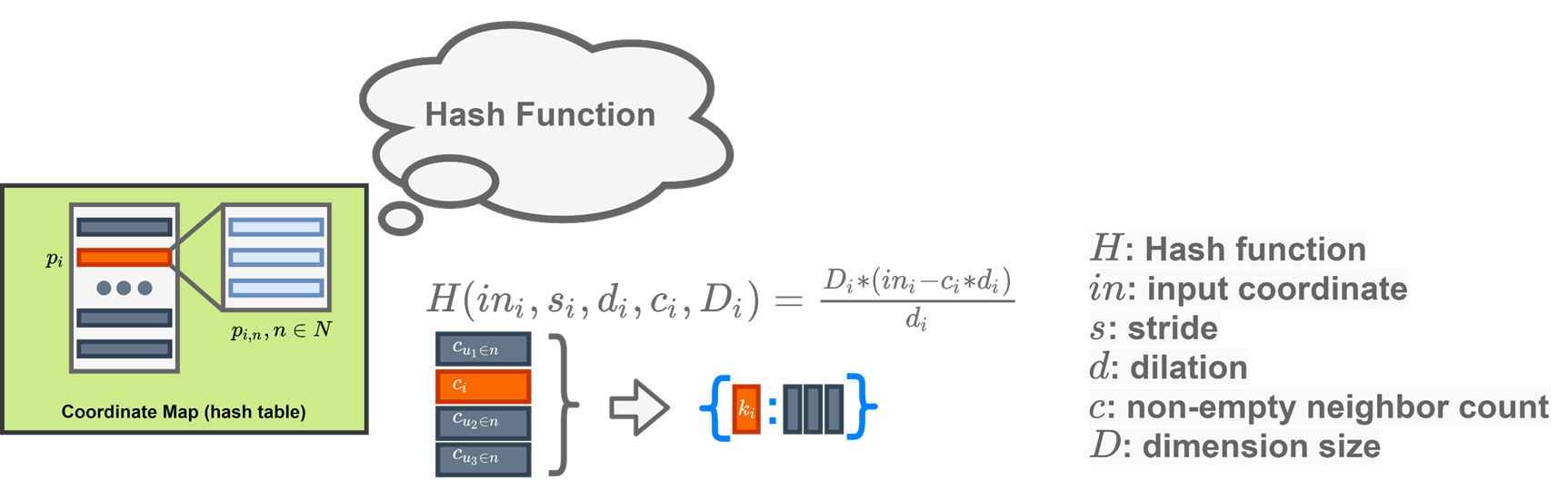
The coordinate mapping will be generate as a dictionary, and stored in memory, when we want to query the neighborhood, we can bring it out to use.

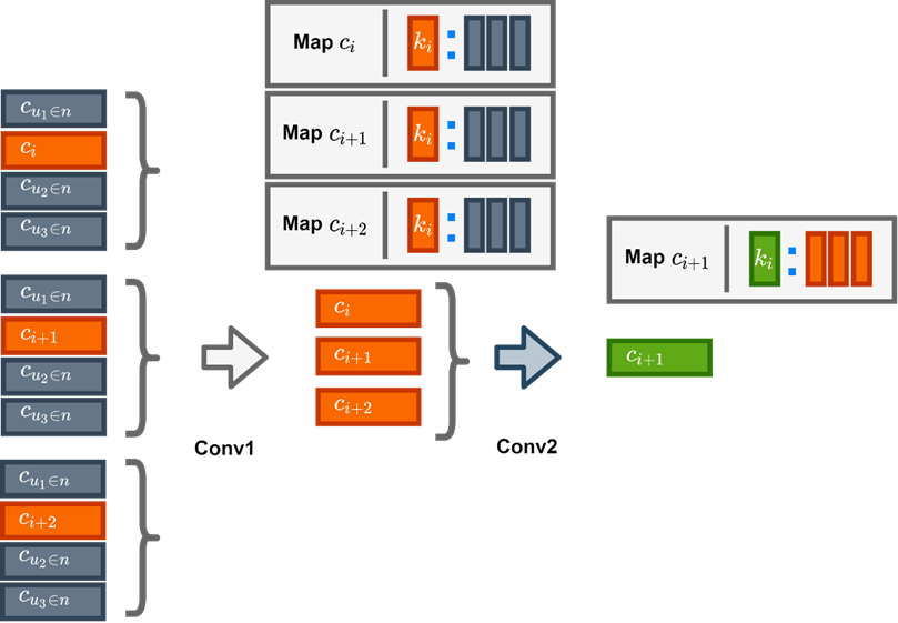
The mapping of different layers are linked hierarchically.

As we can see that if we are not using the coordinate mapping saved from the convolution layer, the internal relationship was broken, and after transpose conv, the coordinate is growing in all directions which covers the whole kernel region.

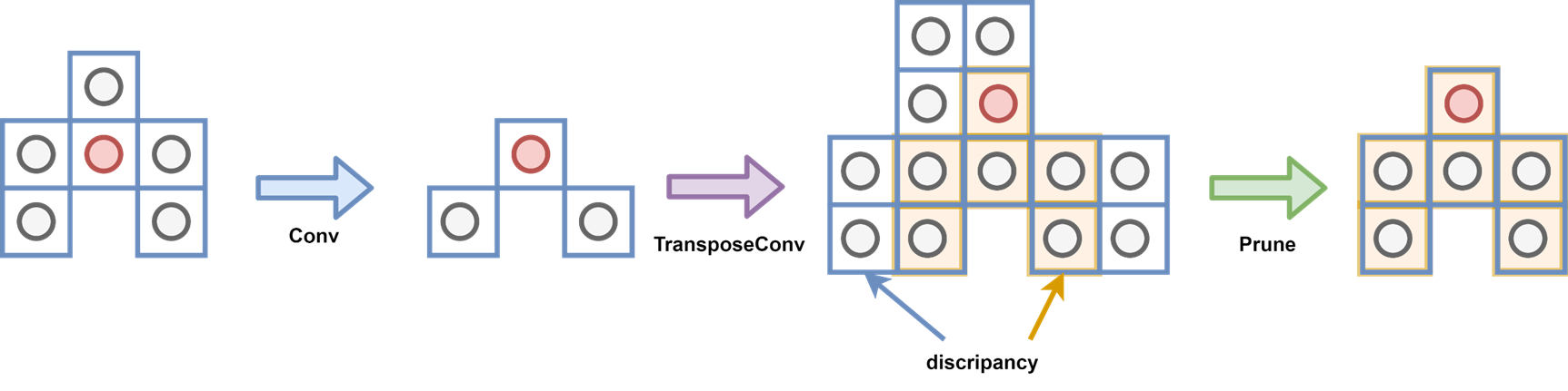
As shown above, the coordinate will be generated more than the original coordinate shape. We need the extra ground truth model to regularize this growth, we can use a prun layer to cut off those extra generated coordinates, and we can also make this layer learnable which is equivalent to teaching a tailor to make the cloth.