
Modern Hopfield Networks, Geometrically: From Wide Memory Basins to Attention
Modern Hopfield Networks can feel mysterious at first because the formulas look simple, but the behavior looks dramatically more powerful than classical Hopfield networks.
This post builds the intuition from geometry.
We will go step by step:
- why classical Hopfield memories interfere,
- why log-sum-exp creates much sharper memory selectivity,
- why that leads to exponential capacity intuition,
- and why the update rule is exactly attention.
Every major idea here is paired with a visualization or animation from the accompanying modern_hopfield demo.
1. The core problem: memory basins merge
A classical Hopfield network stores memories by accumulating them into a single quadratic energy function. Geometrically, each memory direction creates a broad low-energy valley. If two memories are close, those valleys overlap and become one shared basin.
That is the root of interference: the system no longer has two clearly separated destinations.
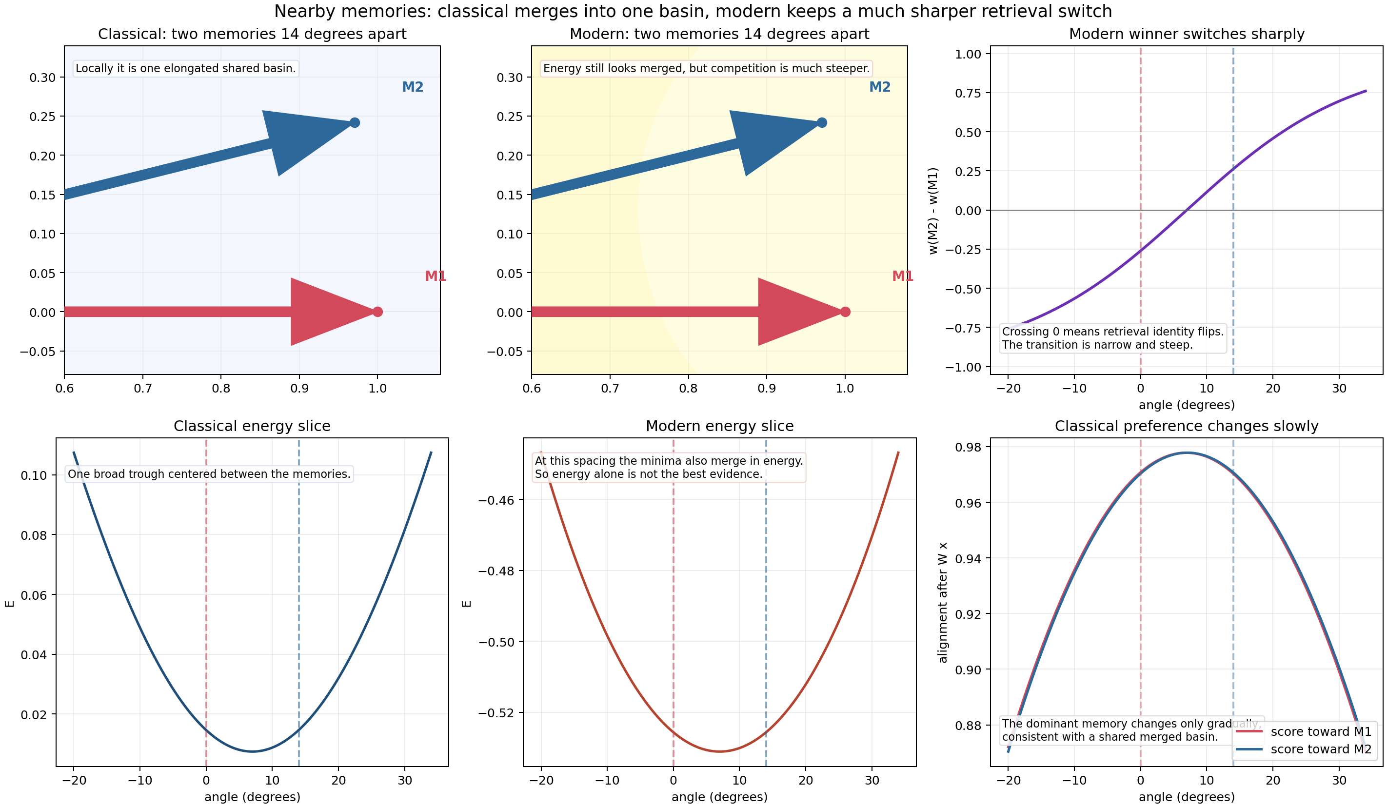
The key takeaway from this figure is subtle but important:
- in the classical case, nearby memories create one broad shared trough;
- in the modern case, the energy can still look merged at this spacing, but the winner switch is much sharper.
That sharper switch is the beginning of modern Hopfield selectivity.
2. Classical Hopfield: one quadratic landscape for everything
The classical energy is
\[E(\mathbf{r}) = -\frac{1}{2N} \sum_{\mu=1}^{P} (\boldsymbol{\xi}^{\mu} \cdot \mathbf{r})^2.\]Each dot product $\boldsymbol{\xi}^{\mu} \cdot \mathbf{r}$ measures how much the current state $\mathbf{r}$ aligns with memory $\boldsymbol{\xi}^{\mu}$. Squaring and negating it means:
- larger projection onto a memory direction lowers energy,
- but every stored memory contributes through the same global quadratic form.
So instead of getting one isolated pocket per memory, you get a smooth low-rank landscape shaped by all memories at once.
In code, the classical matrix is built as an outer-product sum:
def classical_weight_matrix(memories: np.ndarray) -> np.ndarray:
    return memories.T @ memories / memories.shape[1]


def classical_energy(x: np.ndarray, W: np.ndarray) -> float:
    return 0.5 * np.dot(x, x) - 0.5 * np.dot(x, W @ x)
This is exactly why classical storage is global: adding one new memory changes the whole quadratic form.
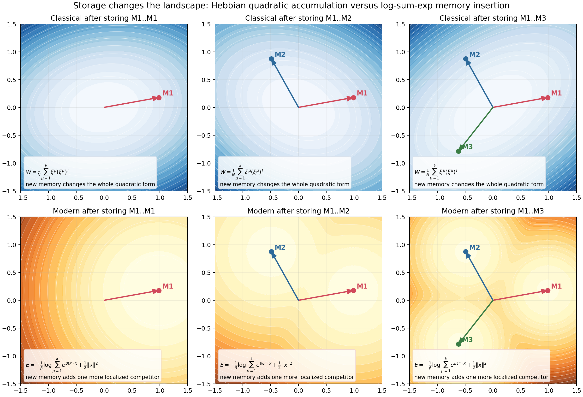
The top row shows classical storage. Each new memory changes the entire energy surface, not just a local region.
You can also compare the global geometry directly:
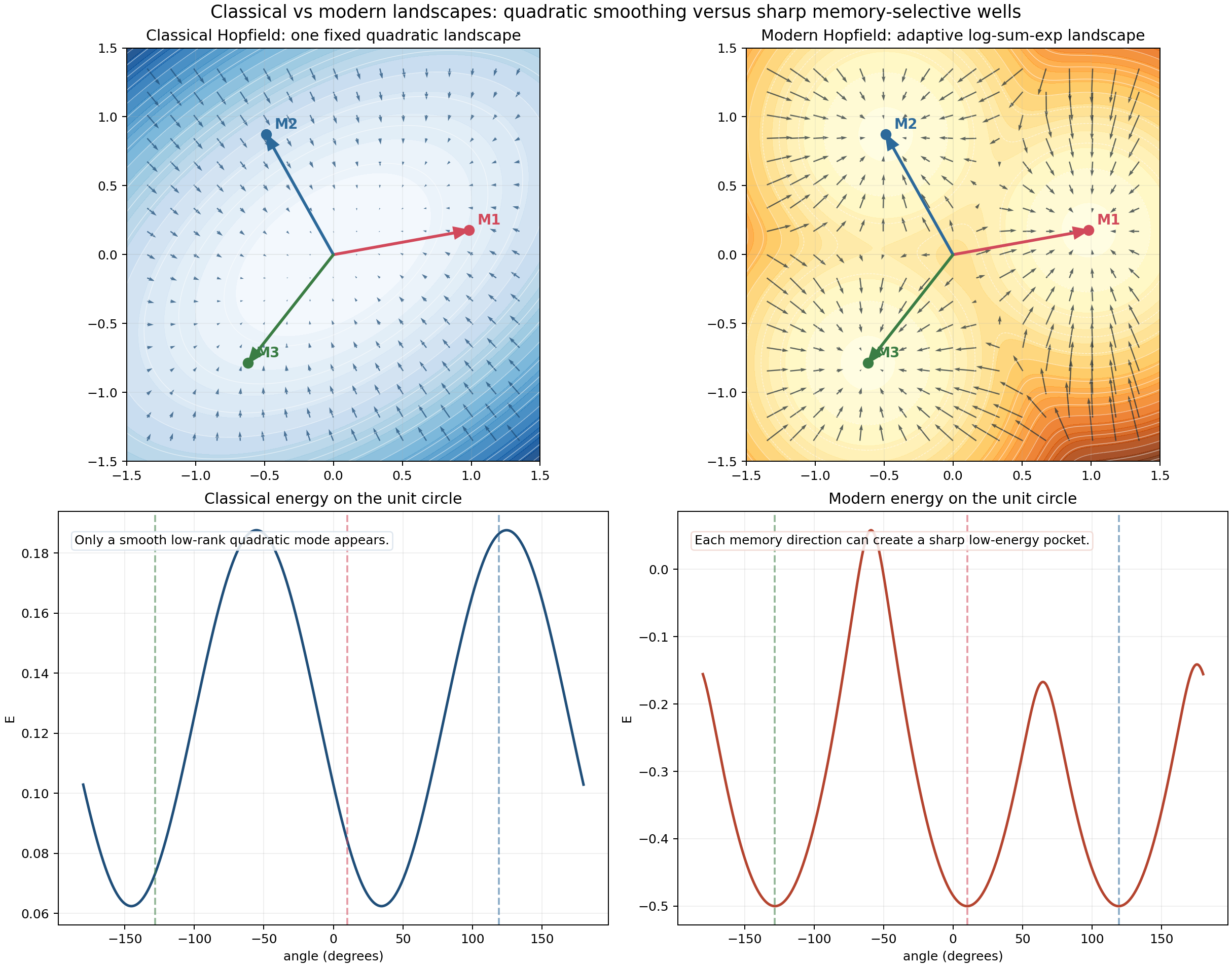
On the classical side, what appears is a broad smooth mode rather than sharply isolated basins.
3. Modern Hopfield: log-sum-exp turns memory competition into soft winner-take-all
Modern Hopfield replaces the quadratic accumulation with
\[E(\mathbf{r}) = -\frac{1}{\beta} \log \sum_{\mu=1}^{P} e^{\beta \boldsymbol{\xi}^{\mu} \cdot \mathbf{r}} + \frac{1}{2}\|\mathbf{r}\|^2.\]Write it in words:
- compute similarity scores between the current state and all memories,
- exponentiate them,
- sum them,
- take a log.
The log-sum-exp term is a smooth max:
\[\max_i z_i \le \log \sum_i e^{z_i} \le \max_i z_i + \log P.\]So when $\beta$ is large, the energy is dominated by the largest score.
This changes the geometry completely.
Instead of “all memories pull comparably,” we get:
- one memory dominates locally,
- the dominant identity can switch sharply,
- and the network behaves much more like a selective retrieval system than a broad averaging system.
The code is compact:
def hopfield_update(x: np.ndarray, memories: np.ndarray, beta: float):
    scores = beta * (memories @ x)
    weights = softmax(scores)
    x_next = weights @ memories
    return scores, weights, x_next


def energy(x: np.ndarray, memories: np.ndarray, beta: float) -> float:
    scores = beta * (memories @ x)
    max_score = np.max(scores)
    logsumexp = max_score + np.log(np.sum(np.exp(scores - max_score)))
    return 0.5 * np.dot(x, x) - logsumexp / beta
That one line
x_next = weights @ memories
already contains most of the modern intuition: the next state is a weighted combination of memories, and the weights come from sharp exponential competition.
A one-dimensional slice makes the difference visible
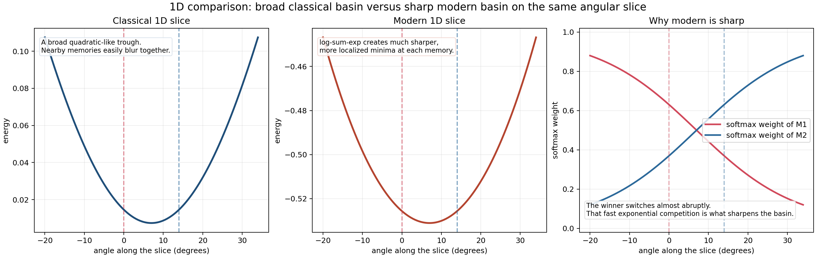
The right panel is the most important one. The softmax weights switch rapidly across a narrow angular region. Even when the energy minimum itself is not visibly split into two separate wells, the retrieval identity changes much more sharply than in the classical case.
4. The update is easier to understand than the energy
A good way to teach modern Hopfield is to stop staring at the formula and ask:
What does one update step do geometrically?
The answer is beautifully concrete.
Step 1: score every memory
For a current state $\mathbf{x}$, compute
\[s_i = \beta \langle \mathbf{x}, M_i \rangle.\]This is just projection onto each memory direction, scaled by $\beta$.
Step 2: convert scores into a competition
\[w_i = \frac{e^{s_i}}{\sum_j e^{s_j}}.\]Now the best-aligned memories get exponentially larger influence.
Step 3: move to the weighted barycenter
\[\mathbf{x}_{\text{next}} = \sum_i w_i M_i.\]So the update lands inside the convex hull of the memories.
That is why modern Hopfield retrieval looks like soft selection among stored prototypes.
The figure below decomposes this carefully.
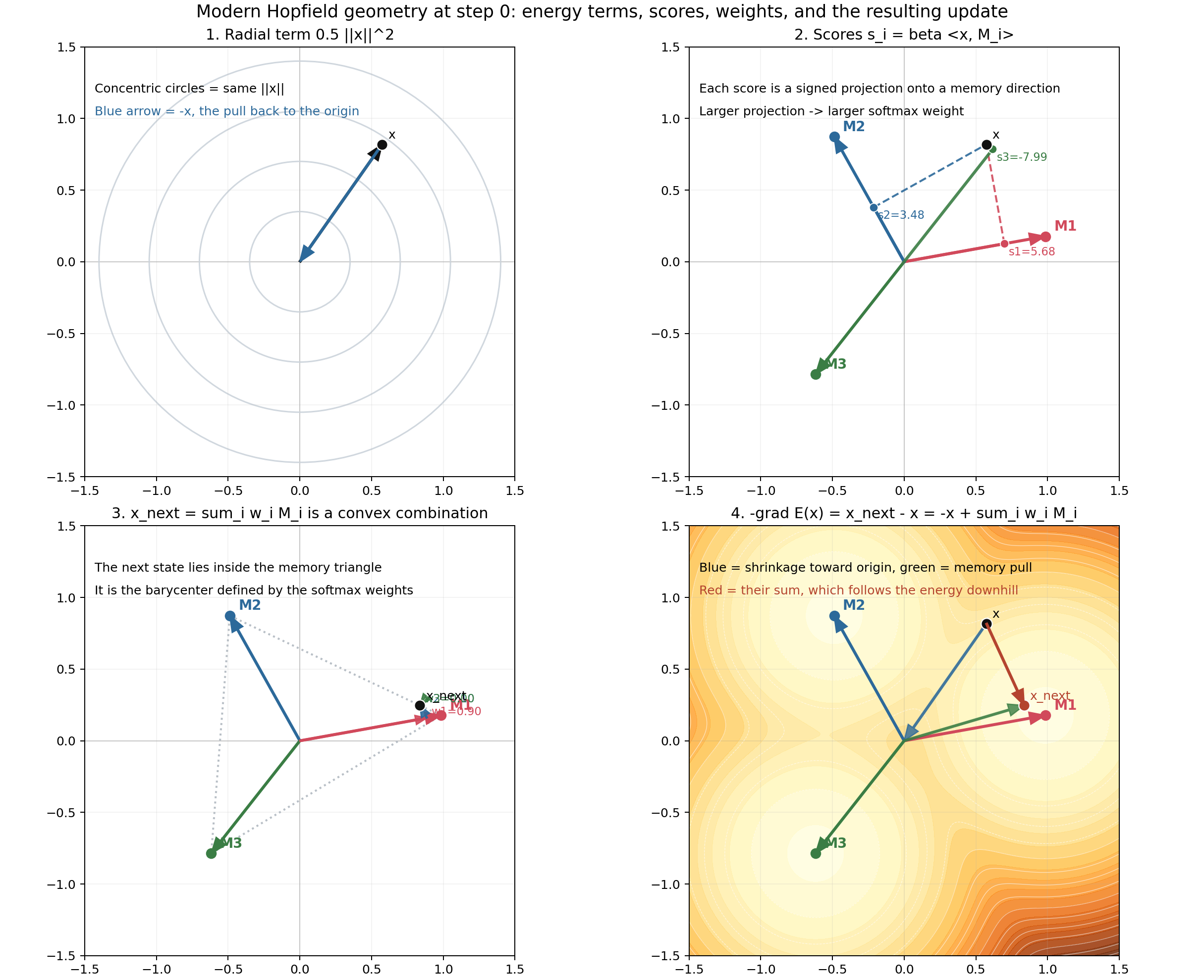
This figure corresponds directly to the main code primitives in matplotlib_walkthrough.py:
projection()for score geometry,softmax()for competition,hopfield_update()for the next state,weighted_covariance()for the local geometry around the selected mixture.
5. Watch the state move: retrieval as downhill motion
The energy landscape is fixed once the memories are stored. Retrieval means the state moves on that landscape.
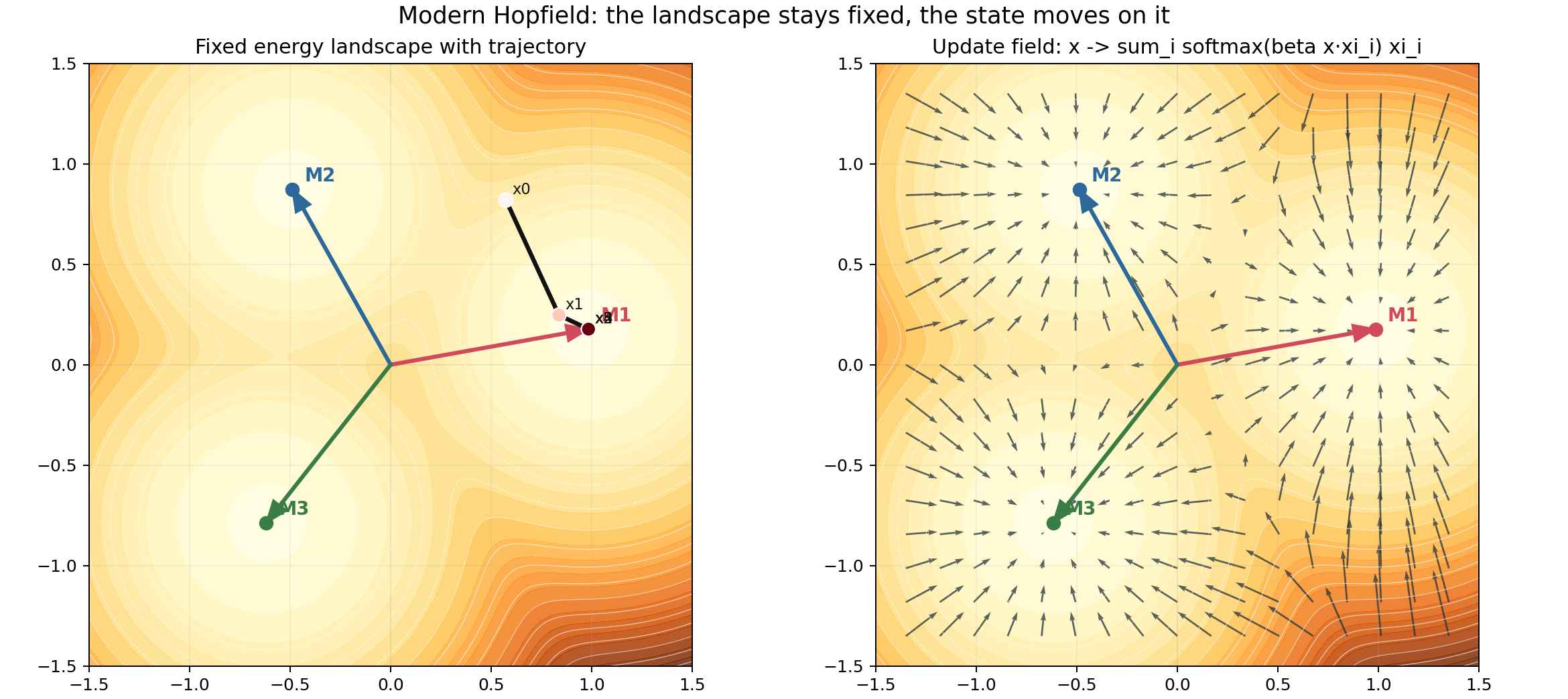
The state does not rebuild the landscape at every step. The contours stay fixed. Only the point moves.
To make this feel intuitive, the demo also generates an animation:
This is the simplest mental model of retrieval:
- the query starts somewhere in state space,
- it scores the memories,
- softmax decides the mixture,
- the point moves,
- and repeated updates slide it into a lower-energy region.
A second animation shows the weights themselves changing through the trajectory.
This is often the most intuitive bridge to attention: retrieval is just similarity-based weighting that evolves as the state becomes more aligned with one memory than the others.
6. Why modern basins feel sharper
A common misunderstanding is to say that modern Hopfield always gives obviously separated “needle wells” in every 2D picture.
That is too strong.
A better statement is:
modern Hopfield creates much sharper competition boundaries and much more localized dominance regions.
The winner-switch animation is designed to show exactly that.
As the query direction moves slightly, the dominant memory flips quickly. That sharp switch is what reduces interference.
By contrast, classical preference changes more gradually, which is consistent with shared merged basins.
You can also compare trajectories directly:
The two systems see the same starting point, but the retrieval geometry is different:
- classical uses a fixed linear map $W x$,
- modern uses adaptive softmax retrieval.
7. Why capacity jumps from linear intuition to exponential intuition
Classical Hopfield capacity is limited because broad basins interfere. If every memory creates a wide valley, you can only fit so many valleys before they overlap badly.
That gives the familiar linear-capacity intuition.
Modern Hopfield changes the failure mode.
A target memory gets score
\[\beta \langle \xi^{\text{target}}, x \rangle,\]while distractor memories get their own scores. In high dimensions, random memories are nearly orthogonal, so their projections concentrate. That means the target score can dominate while distractor scores remain far enough below it for the exponential to suppress them strongly.
The demo includes both a toy empirical retrieval experiment and a schematic scaling intuition:
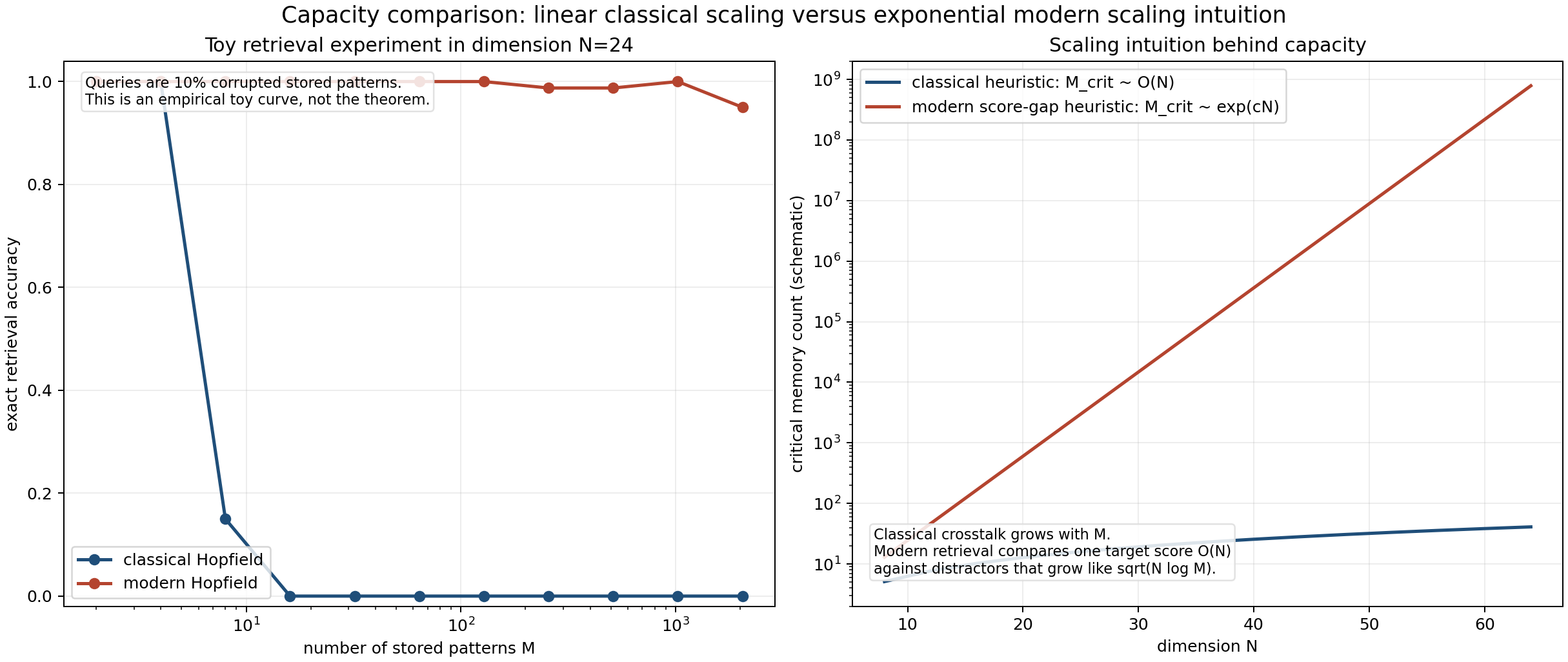
This is not a full proof. It is the geometric takeaway:
- classical fails because crosstalk accumulates in one shared quadratic object,
- modern succeeds because retrieval depends on score gaps passed through exponentials.
That is why the practical intuition becomes exponential in dimension rather than merely linear.
8. The attention connection is not an analogy, it is the same update
Now comes the most important punchline.
The modern Hopfield update is
\[\mathbf{r}^{\text{new}} = X \, \text{softmax}(\beta X^T \mathbf{r}).\]Interpret the symbols:
- current state $\mathbf{r}$ acts like the query,
- stored memory matrix $X$ acts like the keys when computing similarity,
- and also supplies the values in the simplest tied-memory case.
Compare this with attention:
\[\mathrm{Attention}(Q, K, V) = \mathrm{softmax}\!\left(\frac{QK^T}{\sqrt{d_k}}\right) V.\]The mapping is direct:
| Modern Hopfield | Attention |
|---|---|
| state $\mathbf{r}$ | query $Q$ |
| memory matrix in score computation | keys $K$ |
| memory matrix in weighted output | values $V$ |
| $\beta$ | $1/\sqrt{d_k}$ scale |
So attention is not just “similar to associative memory.” It is a modern Hopfield retrieval step.
That is why the idea is best taught geometrically:
- score keys,
- exponentiate competition,
- take a weighted combination of values,
- move to the retrieved prototype or mixture.
In a Transformer, this landscape is rebuilt every forward pass from the current context. In a persistent memory system, the landscape is encoded by stored patterns. But the retrieval rule is the same object.
9. Memory storage: global rewriting versus local competition
The storage difference is as important as the retrieval difference.
In classical Hopfield, storing a new memory modifies the global quadratic matrix:
\[W = \frac{1}{N} \sum_{\mu=1}^{P} \xi^{\mu} (\xi^{\mu})^T.\]In modern Hopfield, storing a new memory means adding one more competitor inside the log-sum-exp term.
That is much closer to the attention viewpoint: memory is not one rigid quadratic object. It is a set of candidates competing through similarity.
The storage animation makes this visible.
The classical landscape changes everywhere because the quadratic form changes everywhere. The modern landscape changes by adding one more localized competitor.
10. The local covariance picture
One underappreciated idea in modern Hopfield geometry is the local covariance of the selected mixture.
In code:
def weighted_covariance(memories: np.ndarray, weights: np.ndarray) -> np.ndarray:
    mean = weights @ memories
    centered = memories - mean
    return (weights[:, None] * centered).T @ centered
This tells you how spread out the currently relevant memories are under the softmax distribution.
- If one memory dominates, covariance is small.
- If several memories compete, covariance grows.
That is a nice way to think about local geometry:
- sharp retrieval means concentrated weights,
- concentrated weights mean smaller local uncertainty,
- and smaller local uncertainty means more memory-specific behavior.
The per-step panel figure shows this with a covariance ellipse:
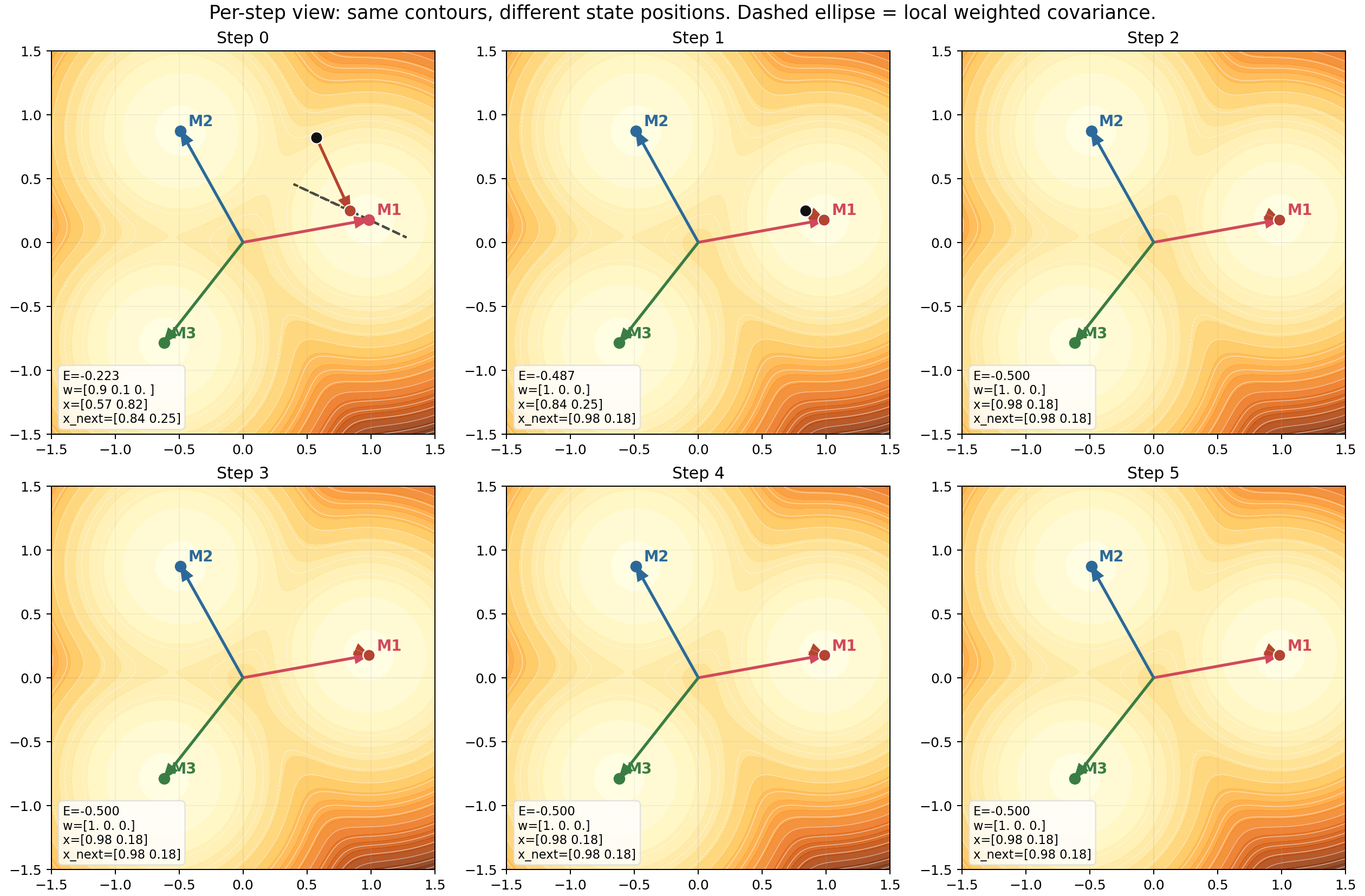
The ellipse is a compact geometric summary of how ambiguous the current retrieval neighborhood is.
11. The complete intuitive story
If you want one short story to remember, use this one:
Classical Hopfield
- stores all memories in one quadratic matrix,
- creates broad smooth basins,
- nearby memories interfere,
- retrieval is a fixed linear map followed by attraction,
- capacity is limited by basin overlap.
Modern Hopfield
- stores memories as competitors inside a log-sum-exp energy,
- creates sharp soft winner-take-all selection,
- reduces interference through exponential score separation,
- retrieval is an adaptive weighted sum of memories,
- and that update is exactly attention.
That is the whole arc from associative memory to Transformers.
12. Run everything yourself
Install dependencies:
python3 -m pip install -r requirements.txt
Generate all static figures:
python3 matplotlib_walkthrough.py --out-dir outputs/figures
Generate static figures plus GIFs:
python3 matplotlib_walkthrough.py --out-dir outputs --generate-gifs
Useful parameters:
python3 matplotlib_walkthrough.py --beta 12 --angle 10 --steps 6 --out-dir outputs
Parameters to explore:
--beta: higher values make the winner switch sharper,--angle: moves the starting query direction,--steps: controls rollout depth,- nearby memory spacing inside
save_nearby_memory_comparison()andsave_winner_switch_animation()controls how difficult retrieval is.
13. Where each idea lives in the code
If you want to read the implementation alongside this post, these are the main anchors:
hopfield_update()for the retrieval step,energy()for the modern Hopfield energy,weighted_covariance()for local geometry,rollout()for repeated retrieval dynamics,- the geometric decomposition figure builder,
- the nearby-memory comparison helper,
- and the GIF generation utilities.
14. Final intuition
The cleanest intuition is not “modern Hopfield has magic capacity.”
It is this:
classical Hopfield stores memories as one shared smooth object, while modern Hopfield turns retrieval into sharp similarity competition.
And the moment you write that competition as
\[\text{softmax}(\text{similarity}) \times \text{values},\]you are already in attention land.
That is why modern Hopfield networks are such a satisfying bridge concept: they connect old associative memory ideas to the core mechanism of Transformers with almost no wasted machinery.