Event-Driven Video Tokens: Porting H-Net's Dynamic Chunking to Hour-Long Robot Video
Abstract. Robot policies would benefit from hours of visual history, but fixed video tokenizers make that impossible: one hour of 10 Hz video is 36,000 frames and roughly 9 million ViT patch tokens. Following Cartesia’s argument that models should learn where to cut their input (part 1, part 2), we port H-Net’s dynamic chunking from bytes to video frames. The result is a causal, action-conditioned, two-level hierarchy whose expensive main network sees only “event” tokens. We pair it with an event-driven streaming engine that runs the main network only when a top-level token is emitted. We study it on a synthetic long-horizon tabletop environment with ground-truth events.
The systems claims hold. Streaming is numerically identical to the training-time forward pass. The main network’s share of per-frame compute drops from 85% to 0.3–4%. Main-network KV after one hour shrinks from 590 MB to 2–26 MB. At a realistic 680M-parameter scale, a full day of video needs 1–6 GB instead of 127 GB.
The learning claims do not hold yet. The learned router’s boundary probability collapses onto its decision threshold, so its boundaries are no better aligned with action events than random ones. A long-range memory task stays at chance for every model, including uncompressed full attention, because the objective never rewards remembering. We trace both failures to specific, fixable causes and lay out the next experiments.
摘要。 机器人策略如果能看到几个小时的视觉历史,会受益很多,但固定的视频 tokenizer 让这件事根本做不到:10 Hz 的视频一小时就是 36,000 帧,换成 ViT patch token 大约是 900 万个。Cartesia 认为模型应该自己学会在哪里切分输入(第一篇、第二篇)。顺着这个思路,我们把 H-Net 的动态分块从字节搬到视频帧上,得到一个因果的、以动作为条件的两层层级结构,其中昂贵的主网络只看「事件」token。我们还配了一个事件驱动的流式引擎,只在顶层发出 token 时才运行主网络。整个系统在一个带事件真值的合成长时程桌面环境上做了研究。
系统层面的结论成立。 流式推理与训练时的整段前向在数值上完全一致。主网络在每帧计算量中的占比从 85% 降到 0.3–4%。一小时后主网络的 KV 从 590 MB 降到 2–26 MB。按 6.8 亿参数的真实规模推算,一整天的视频只要 1–6 GB,而不是 127 GB。
学习层面的结论暂不成立。 学出来的 router 的边界概率塌缩到了判决阈值上,导致它的边界与动作事件的对齐程度并不比随机边界好。一个长程记忆任务在所有模型上都停在随机水平,包括不压缩的全注意力模型,因为目标函数从不奖励「记住」。我们把这两个失败分别追溯到了具体、可修复的原因,并给出了下一步实验。
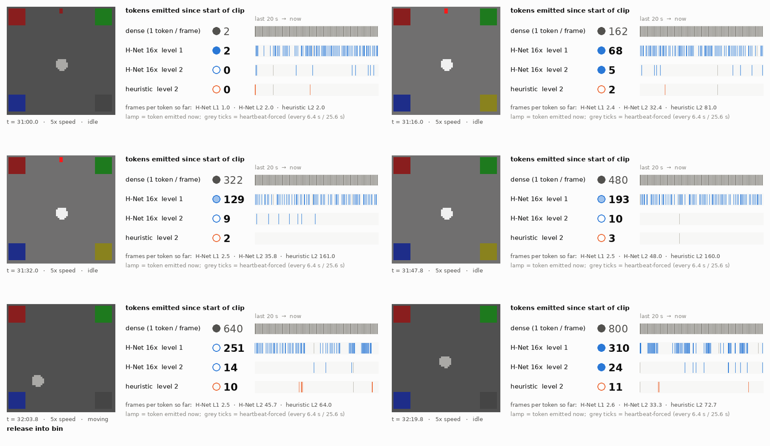
Figure 1. A held-out stream from the synthetic tabletop environment (5× speed). The counters compare a dense tokenizer (one token per frame) with level 1 and level 2 of the learned hierarchy and a pixel-change heuristic.
图 1. 合成桌面环境中一段未参与训练的视频流(5 倍速)。计数器对比了稠密 tokenizer(每帧一个 token)、学习得到的层级结构第一层与第二层,以及一个基于像素变化的启发式方法。
1. Introduction
A policy that conditions on a few frames cannot remember where it put an object, whether a sub-task already failed, or what an operator showed it ten minutes ago. Extending the visual context is conceptually simple and computationally prohibitive:
| tokenizer | tokens / frame | 1 h | 24 h |
|---|---|---|---|
| ViT patches, 224² | 256 | 9.2 M | 221 M |
| pooled VLM tokens | 64 | 2.3 M | 55 M |
| one vector per frame | 1 | 36 K | 864 K |
| event tokens (ours) | adaptive | 0.14–2.3 K | 3.4–54 K* |
10 Hz video. *1 h is measured; 24 h is 24 × the hourly rate. A measured 24 h stream gave 45 K tokens for learned 16×.
Fixed tokenizers allocate the same budget to every frame. Robot streams are the opposite of uniform. In our environment 68% of frames are idle, and the decision-relevant moments are sparse: contacts, grasps, failures, scene changes.
Byte-level language modelling has the same structure. Cartesia’s H-Net results show that learned, end-to-end dynamic chunking beats both BPE and entropy-threshold patching (BLT) at matched compute, and that hand-designed segmentation is a prior worth removing.
We ask three questions:
- RQ1 (systems). If chunking is learned and causal, can we run the expensive part of the model only at the event rate, and what does that buy in memory and compute over an hour or a day?
- RQ2 (allocation). Does a learned router put its tokens on action-relevant events, rather than on whatever is visually loud?
- RQ3 (memory). Does the compressed history support decisions that depend on the far past?
The answers turn out to be yes, not yet, and not yet. The two negative answers are the more informative ones.
1. 引言
只看几帧的策略,记不住自己把物体放在了哪、某个子任务是不是已经失败过、操作员十分钟前给它演示了什么。扩展视觉上下文在概念上很简单,在算力上却做不到:
| tokenizer | 每帧 token | 1 小时 | 24 小时 |
|---|---|---|---|
| ViT patch,224² | 256 | 920 万 | 2.21 亿 |
| 池化后的 VLM token | 64 | 230 万 | 5,500 万 |
| 每帧一个向量 | 1 | 3.6 万 | 86.4 万 |
| 事件 token(本文) | 自适应 | 0.14–2.3 千 | 0.34–5.4 万* |
10 Hz 视频。*1 小时为实测;24 小时为每小时速率 × 24。learned 16× 在一条 24 小时视频流上实测为 4.5 万。
固定 tokenizer 给每一帧分配同样的预算,而机器人视频流恰恰最不均匀:在我们的环境里 68% 的帧是空闲的,与决策相关的时刻很稀疏,包括接触、抓取、失败和场景变化。
字节级语言建模也是同样的结构。Cartesia 的 H-Net 结果表明,在同等算力下,端到端学习的动态分块既胜过 BPE,也胜过基于熵阈值的切块(BLT),而人工设计的切分方式是一个值得去掉的先验。
我们问三个问题:
- RQ1(系统)。 如果分块是学出来的、而且是因果的,能不能让模型里昂贵的那部分只按事件速率运行?在一小时、一天的尺度上,这能换来多少显存和算力?
- RQ2(分配)。 学出来的 router 会把 token 放在与动作相关的事件上,而不是放在视觉上「动静大」的地方吗?
- RQ3(记忆)。 压缩后的历史能支撑依赖遥远过去的决策吗?
答案分别是:能;还不行;还不行。后两个否定的答案,信息量反而更大。
2. Background: dynamic chunking in H-Net
H-Net (Hwang, Wang & Gu, 2025) is a recursive encoder–main-network–decoder. Light outer layers process every position, and a routing module scores each position by the dissimilarity to its predecessor:
\[q_t = W_q h_t,\qquad k_t = W_k h_t,\] \[p_t = \tfrac{1}{2}\bigl(1 - \cos(q_t, k_{t-1})\bigr),\qquad b_t = \mathbb{1}[p_t \ge \tfrac12].\]Positions with $b_t = 1$ are gathered into a shorter sequence for the main network. A ratio loss steers the boundary rate towards a target $1/N$ using the hard fraction $F = \tfrac1T\sum_t b_t$ and the soft fraction $G = \tfrac1T\sum_t p_t$:
\[\mathcal{L}_{\text{ratio}} = \frac{N}{N-1}\Bigl[(N-1)\,F\,G + (1-F)(1-G)\Bigr].\]On the way back down, chunk outputs $z_k$ are smoothed with an EMA gated by the boundary probability, which is what gives the discrete router a gradient:
\[\bar z_k = P_k\, z_k + (1 - P_k)\,\bar z_{k-1}.\]Each position receives the most recent smoothed chunk, scaled by a straight-through confidence, plus a residual from its own encoder:
\[y_t = \bar z_{c(t)}\cdot \mathrm{STE}(c_t) + W_r h_t,\] \[c_t = p_t^{\,b_t}(1-p_t)^{1-b_t}.\]Because the main network can itself be an H-Net, compression is hierarchical.
2. 背景:H-Net 中的动态分块
H-Net(Hwang、Wang 与 Gu,2025)是一个递归的「编码器 – 主网络 – 解码器」结构。轻量的外层处理每一个位置,一个路由模块(routing module)根据每个位置和前一个位置的差异给它打分:
\[q_t = W_q h_t,\qquad k_t = W_k h_t,\] \[p_t = \tfrac{1}{2}\bigl(1 - \cos(q_t, k_{t-1})\bigr),\qquad b_t = \mathbb{1}[p_t \ge \tfrac12].\]$b_t = 1$ 的位置被收集成一条更短的序列,交给主网络。比率损失(ratio loss)用硬比例 $F = \tfrac1T\sum_t b_t$ 和软比例 $G = \tfrac1T\sum_t p_t$,把边界率引向目标 $1/N$:
\[\mathcal{L}_{\text{ratio}} = \frac{N}{N-1}\Bigl[(N-1)\,F\,G + (1-F)(1-G)\Bigr].\]往回走时,chunk 的输出 $z_k$ 经过一个由边界概率门控的 EMA 平滑,这正是离散 router 能拿到梯度的原因:
\[\bar z_k = P_k\, z_k + (1 - P_k)\,\bar z_{k-1}.\]每个位置拿到最近一个平滑后的 chunk,乘上一个直通估计(straight-through)的置信度,再加上来自它自己编码器的残差:
\[y_t = \bar z_{c(t)}\cdot \mathrm{STE}(c_t) + W_r h_t,\] \[c_t = p_t^{\,b_t}(1-p_t)^{1-b_t}.\]由于主网络本身也可以是一个 H-Net,压缩是分层进行的。
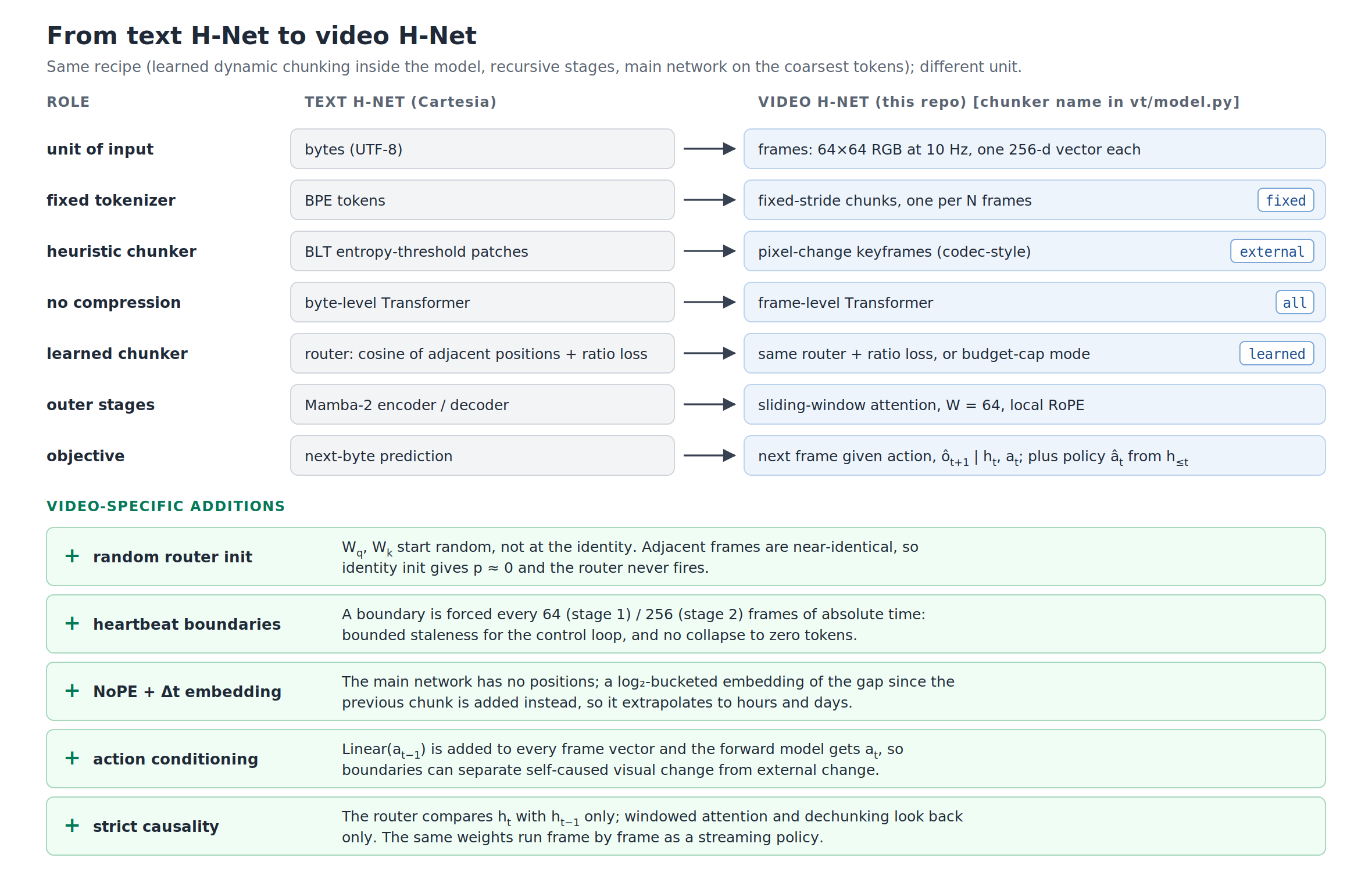
Figure 2. Mapping the text setting onto video. Each baseline in Cartesia’s study has a direct video analogue: BPE becomes a fixed temporal stride, BLT’s entropy threshold becomes a pixel-change (keyframe) threshold, and the byte Transformer becomes a frame Transformer.
3. Method
3.1 Frames as bytes
Each 64×64 RGB frame $o_t$ is encoded by a small CNN into one 256-d vector. We add an embedding of the previous action $a_{t-1}$ to it, so the stream the router sees is proprioceptively aware. Two H-Net stages follow:
- Level 1 has width 256, two sliding-window attention blocks with a 64-frame window, and a target of about 1 token per 4 frames.
- Level 2 has width 384 and a target of about 1 token per 16–23 frames.
- The main network is 8 full-causal attention blocks at width 512. Its KV cache is the model’s long-term memory.
Tokens are continuous vectors with timestamps, not codebook indices. For a live stream, the tokenizer’s output is a ragged list ${(z_k, t_k)}$.
图 2. 把文本设定映射到视频上。Cartesia 研究中的每个基线在视频里都有直接对应:BPE 对应固定的时间步长,BLT 的熵阈值对应像素变化(关键帧)阈值,字节级 Transformer 对应逐帧 Transformer。
3. 方法
3.1 把帧当作字节
每张 64×64 的 RGB 帧 $o_t$ 由一个小 CNN 编码成一个 256 维向量。我们在上面加上前一个动作 $a_{t-1}$ 的 embedding,这样 router 看到的序列是带本体感知的。后面接两个 H-Net 阶段:
- 第一层宽度 256,两个滑动窗口注意力块(窗口 64 帧),目标约每 4 帧 1 个 token。
- 第二层宽度 384,目标约每 16–23 帧 1 个 token。
- 主网络是 8 个全因果注意力块,宽度 512,它的 KV cache 就是模型的长期记忆。
token 是带时间戳的连续向量,而不是码本索引。对一条实时视频流来说,tokenizer 的输出就是一个长短不一的列表 ${(z_k, t_k)}$。
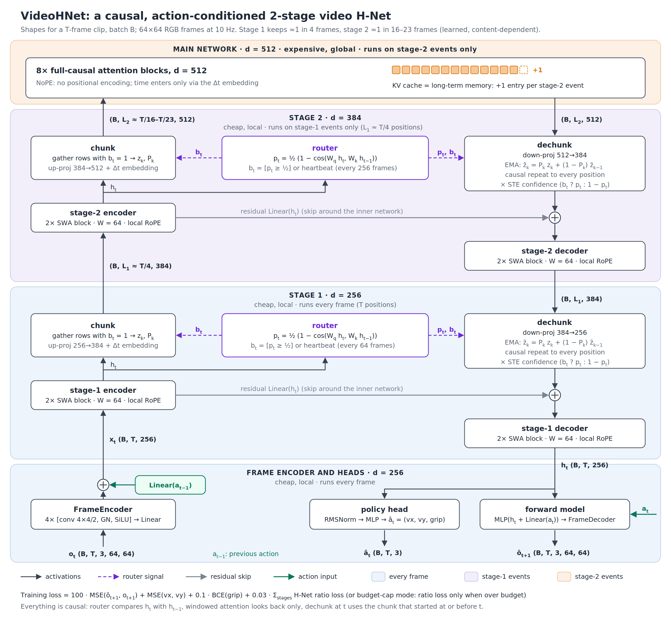
Figure 3. Architecture. Blue regions run every frame, purple ones only on level-1 events, and orange ones only on level-2 events. Shapes are given for a T-frame clip.
3.2 Modifications required for video and control
Four changes were necessary before the model trained at all.
- Router initialisation. H-Net initialises $W_q = W_k = I$. On text, adjacent bytes differ enough for this to produce boundaries. On video, adjacent frames are nearly identical, so $\cos \approx 1$, $p_t \approx 0$, and no boundary is ever emitted: a 2,048-frame clip collapsed into one chunk. We use independent random initialisation instead. Section 6.1 shows that this choice causes the second failure mode.
- Heartbeat boundaries. We force $b_t = 1$ whenever absolute time crosses a multiple of $M_\ell$ ($M_1 = 64$ and $M_2 = 256$ frames). This bounds the staleness of the main network’s view, which a controller needs, and it prevents collapse to zero tokens. It costs $36{,}000/M_\ell$ tokens per hour.
- Time-aware main network. Chunks arrive at irregular intervals, so token index carries no meaning. The main network therefore uses no positional encoding (NoPE). Instead it adds a log-bucketed embedding of $\Delta t_k = t_k - t_{k-1}$. Positions never leave the training distribution, so the model extrapolates from 3-minute training clips to hour- and day-long streams.
- Action-causal objective. A policy head predicts $a_t$, and an action-conditioned forward model predicts $o_{t+1}$ from $(h_{\le t}, a_t)$:
We also test a budget-cap variant. It charges the ratio loss only when over budget and adds a small per-token rate cost, $\mathcal{L}{\text{cap}} = \mathcal{L}{\text{ratio}}\,\mathbb{1}[F > 1/N] + \lambda G$. Below the cap, tokens should be spent only where prediction pays for them.
Every component is strictly causal. The router compares $t$ with $t-1$, attention only looks back, and the dechunker at $t$ uses only a chunk that began at or before $t$. A unit test verifies that perturbing inputs after $t$ leaves every output before $t$ unchanged.
图 3. 模型结构。蓝色区域每帧运行,紫色只在第一层事件时运行,橙色只在第二层事件时运行。图中给出的是 T 帧片段对应的张量形状。
3.2 为视频和控制所做的修改
在模型能训练起来之前,有四处改动是必须的。
- router 初始化。 H-Net 把 $W_q = W_k = I$。在文本上,相邻字节差别够大,这样初始化能产生边界。在视频上,相邻两帧几乎相同,于是 $\cos \approx 1$、$p_t \approx 0$,一个边界都不会产生:一段 2,048 帧的片段塌缩成了一个 chunk。我们改用相互独立的随机初始化。第 6.1 节会说明,正是这个选择导致了第二种失败模式。
- 心跳边界。 绝对时间每跨过 $M_\ell$ 的整数倍($M_1 = 64$、$M_2 = 256$ 帧),就强制 $b_t = 1$。这给主网络视野的陈旧程度设了上限,这是控制器需要的;同时也防止塌缩到零个 token。代价是每小时 $36{,}000/M_\ell$ 个 token。
- 感知时间的主网络。 chunk 到达的间隔不规则,token 序号因此没有意义。所以主网络不用位置编码(NoPE),而是加一个按 log 分桶的 $\Delta t_k = t_k - t_{k-1}$ 的 embedding。位置永远不会离开训练分布,模型因此能从 3 分钟的训练片段外推到小时级、天级的视频流。
- 动作因果的目标函数。 策略头预测 $a_t$;以动作为条件的前向模型由 $(h_{\le t}, a_t)$ 预测 $o_{t+1}$:
我们还测试了一个预算上限(budget-cap)变体:只在超出预算时才施加 ratio loss,另外加一个很小的按 token 计的成本,$\mathcal{L}{\text{cap}} = \mathcal{L}{\text{ratio}}\,\mathbb{1}[F > 1/N] + \lambda G$。在上限以下,token 应当只花在预测能从中获益的地方。
所有组件都是严格因果的:router 比较 $t$ 与 $t-1$,注意力只往回看,第 $t$ 帧的反分块只用在 $t$ 或之前开始的 chunk。一个单元测试验证了:扰动 $t$ 之后的输入,不会改变 $t$ 之前的任何输出。
3.3 Event-driven streaming engine
Causality lets the same weights run one frame at a time. The engine executes the hierarchy lazily:
- Every frame: frame encoder, level-1 encoder/router/decoder, and heads, using a 64-step sliding KV window.
- On a level-1 token: one level-2 step.
- On a level-2 token: one main-network step and one KV-cache append.
Between boundaries, each level reuses its cached smoothed state $\bar z$, which is exactly the quantity dechunking computes in training. In fp32, with TF32 disabled, streaming reproduces the full-sequence forward to a maximum error of $1.6\times10^{-5}$, with identical boundaries, for every chunker type. With TF32 enabled, the error is about $10^{-2}$, because cuDNN selects different convolution algorithms for one frame than for a batch. Anyone building a similar engine should test with TF32 off.
3.3 事件驱动的流式引擎
因果性让同一套权重可以一帧一帧地运行。引擎按需执行层级结构:
- 每一帧:帧编码器、第一层的编码器 / router / 解码器,以及输出头,配一个 64 步的滑动 KV 窗口。
- 第一层发出 token 时:第二层走一步。
- 第二层发出 token 时:主网络走一步,KV cache 追加一条。
在两个边界之间,每一层复用自己缓存的平滑状态 $\bar z$,这正是训练时反分块所计算的量。在 fp32 且关闭 TF32 的情况下,对所有类型的分块器,流式结果都以最大误差 $1.6\times10^{-5}$ 复现整段前向,边界完全相同。若开启 TF32,误差约为 $10^{-2}$,原因是 cuDNN 对单帧和对整批选择了不同的卷积算法。做类似引擎的人,测试时应关闭 TF32。
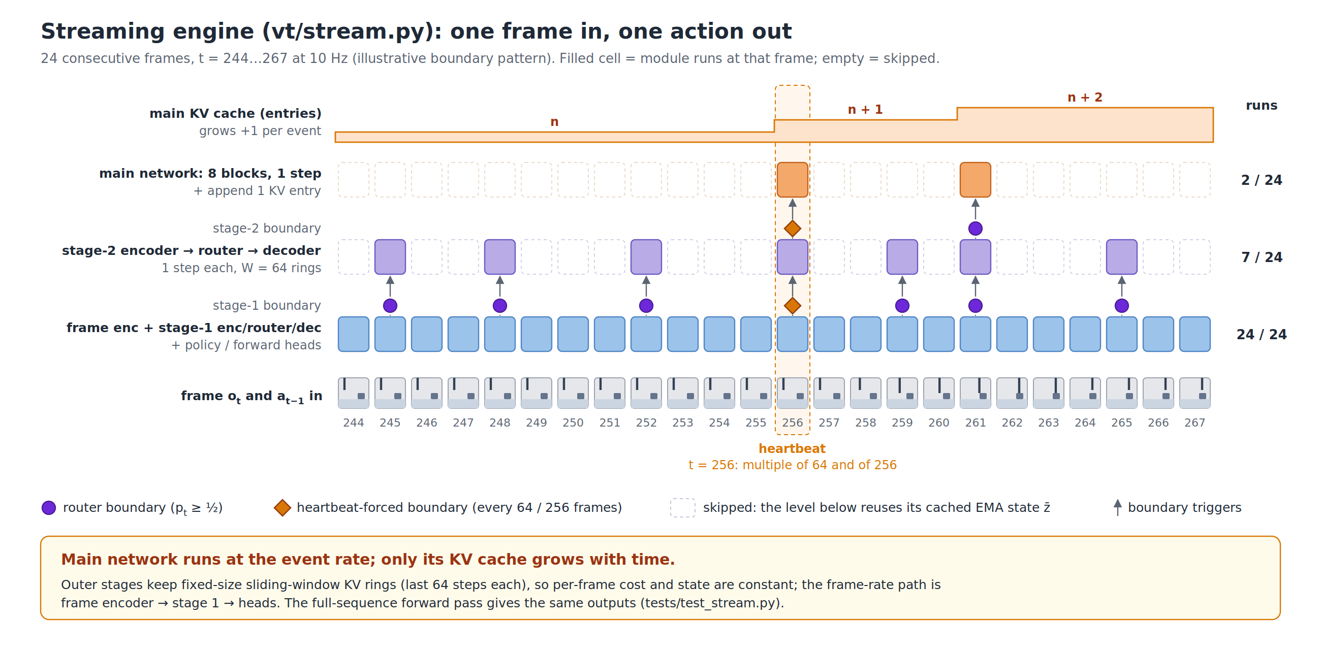
Figure 4. Module schedule of the streaming engine over 24 frames (illustrative boundary pattern). Only the main network’s KV cache grows with time.
4. Experimental setup
Environment. A top-down tabletop rendered at 64×64 and 10 Hz with full ground truth. An end-effector picks blocks and places each one in the bin of its colour. The stream is designed to separate good token allocation from bad:
| property | rate | what it tests |
|---|---|---|
| idle frames (stretches up to 2.5 min) | 68% of frames | can idle time cost ~0 tokens? |
| pick-and-place cycles | ~230 / h | action events that should be tokenized |
| exogenous light toggles | ~100 / h | large pixel change, irrelevant to the next action |
| blinking LED, noise σ = 0.02 | always | predictable nuisance |
| cue → query memory task | ~25 / h | correct action depends only on the far past |
Baselines, all at matched compression where applicable:
- an isotropic frame Transformer with no compression (
dense); - fixed temporal stride (
fixed); - a pixel-change threshold calibrated to the same average rate (
heuristic, the analogue of BLT’s entropy threshold); - learned dynamic chunking at 4×, 16× and 64× (
learned).
Ablations: no action conditioning (video-only), budget cap, long-context fine-tuning, and anti-copycat training.
Protocol. About 40M parameters, 4,000 steps, batch 4 × 2,048 frames, AdamW (6e-4, cosine), bf16, about 11 minutes per run on one RTX 4090. Evaluation is a single causal pass over six held-out one-hour streams, plus a 24-hour stream.
Metrics:
- next-frame PSNR on frames that change, compared with a copy-last-frame baseline;
- action MSE while moving;
- memory recall at query frames (chance is 25%);
- event recall within ±3 frames, compared with random boundaries at the same rate, $1-(1-r)^{7}$;
- tokens per minute in idle versus active segments;
- FLOPs per frame, KV bytes, and latency.
5. Results
5.1 Systems: compute and memory scale with events (RQ1)
We streamed one held-out hour frame by frame through every model and counted FLOPs and state.
图 4. 流式引擎在 24 帧上的模块调度(边界模式为示意)。只有主网络的 KV cache 随时间增长。
4. 实验设置
环境。 一个俯视的桌面场景,64×64、10 Hz 渲染,所有东西都有真值。末端执行器把方块捡起,放进同颜色的筐里。这条视频流专门设计来区分 token 分配的好坏:
| 属性 | 频率 | 检验的是什么 |
|---|---|---|
| 空闲帧(最长持续 2.5 分钟) | 占 68% 的帧 | 空闲时间能否几乎不花 token? |
| 抓放循环 | 约 230 次 / 小时 | 应该被 token 化的动作事件 |
| 外部开关灯 | 约 100 次 / 小时 | 像素变化大,与下一个动作无关 |
| 闪烁的 LED、传感器噪声 σ = 0.02 | 持续 | 可预测的干扰 |
| 提示 → 询问的记忆任务 | 约 25 次 / 小时 | 正确动作只取决于遥远的过去 |
基线,凡适用之处都在同等压缩率下比较:
- 不压缩的各向同性逐帧 Transformer(
dense); - 固定时间步长(
fixed); - 校准到相同平均速率的像素变化阈值(
heuristic,对应 BLT 的熵阈值); - 4×、16×、64× 的学习式动态分块(
learned)。
消融:去掉动作条件(video-only)、预算上限、长上下文微调、反 copycat 训练。
流程。 约 4000 万参数,4,000 步,batch 为 4 × 2,048 帧,AdamW(6e-4,余弦退火),bf16,每次在一张 RTX 4090 上约 11 分钟。评测是在六条未参与训练的一小时视频流上做一次因果前向,外加一条 24 小时的视频流。
指标:
- 变化帧上的下一帧 PSNR,与「复制上一帧」基线对比;
- 运动时的动作 MSE;
- 询问帧上的记忆召回率(随机为 25%);
- ±3 帧内的事件召回率,与同速率随机边界的召回 $1-(1-r)^{7}$ 对比;
- 空闲与活跃片段中每分钟的 token 数;
- 每帧 FLOPs、KV 字节数和延迟。
5. 结果
5.1 系统:算力与显存随事件伸缩(RQ1)
我们把一段未参与训练的一小时视频流一帧一帧地喂给每个模型,统计 FLOPs 和状态大小。
Figure 5 (interactive). Measured streaming cost over one hour.
In the dense model, the main network accounts for 84.5% of per-frame compute. With event-driven execution it falls to 4.0% (16×), 0.7% (64×) and 0.3% (budget cap). Total compute per frame drops by 5.8–6.4×. Main-network KV after one hour is 590 MB dense, compared with 26 MB at 16× and 2.3 MB at the heartbeat floor, and it grows with events rather than frames.
The remaining cost is almost entirely the per-frame frame encoder, about 56 MFLOP per frame. At deployment scale this would be a ViT on every frame of every camera, which makes it the next target for sparsification (Section 8). Latency is 2–3 ms per frame for all models. That is launch-bound at this size and 30–50× inside the 100 ms real-time budget.
To extrapolate beyond the toy scale, we timed one decoding step of a 680M-parameter main network (d = 1536, 24 layers, bf16) on the 4090 at different KV lengths. It takes 3.1 ms at 1K cached tokens, 8.8 ms at 36K and 19.2 ms at 100K. Figure 6 combines these timings with the measured event rates.
图 5(可交互)。一小时流式推理的实测开销。
在稠密模型中,主网络占每帧计算量的 84.5%;改为事件驱动后,降到 4.0%(16×)、0.7%(64×)和 0.3%(预算上限)。每帧总计算量下降 5.8–6.4 倍。一小时后主网络的 KV:稠密为 590 MB,16× 为 26 MB,心跳下限为 2.3 MB,而且随事件增长、不随帧数增长。
剩下的开销几乎全是每帧都跑的帧编码器,约每帧 56 MFLOP。到了部署规模,这就是每个相机、每一帧都跑一次 ViT,所以它是下一个要稀疏化的对象(第 8 节)。所有模型的延迟都是每帧 2–3 ms:在这个规模下受限于 kernel 启动开销,比 100 ms 的实时预算快 30–50 倍。
为了外推到玩具规模之外,我们在 4090 上测了一个 6.8 亿参数主网络(d = 1536,24 层,bf16)在不同 KV 长度下走一步的时间:1K 个缓存 token 时 3.1 ms,36K 时 8.8 ms,100K 时 19.2 ms。图 6 把这些时间和实测的事件速率结合在一起。
Figure 6 (interactive). Real-scale projection on one RTX 4090. The per-step latencies and the event rates are measured; the curves are projections from them.
At one token per frame, a dense model needs 127 GB of KV for a day. At 16 tokens per frame it exceeds 24 GB in well under an hour. At the measured event rates, the event-driven model needs 1–6 GB for a full day, and its main network costs seconds of GPU time per hour of video. RQ1: yes.
5.2 Prediction quality is insensitive to compression
Next-frame PSNR on dynamic frames lies between 35.3 and 35.7 dB for every run, against 29.4 dB for copying the last frame. Action MSE lies between 0.013 and 0.016 for every action-conditioned run. Both are flat from 1× to 255× compression. The local outer stages, with their 64-frame window and residual path, model the short-range dynamics by themselves, so these metrics cannot separate the chunkers. That observation matters again in Section 6.
图 6(可交互)。一张 RTX 4090 上的真实规模推算。每步延迟和事件速率是实测的,曲线是在它们基础上的推算。
每帧 1 个 token 的稠密模型,一天需要 127 GB 的 KV;每帧 16 个 token 时,远不到一小时就超过 24 GB。按实测事件速率运行的事件驱动模型,一整天只要 1–6 GB,主网络每小时视频只花几秒 GPU 时间。RQ1:能。
5.2 预测质量对压缩不敏感
所有模型在变化帧上的下一帧 PSNR 都在 35.3–35.7 dB 之间,「复制上一帧」基线是 29.4 dB。所有带动作条件的模型,动作 MSE 都在 0.013–0.016 之间。两者从 1× 到 255× 压缩都是平的。外层的局部阶段靠 64 帧的窗口和残差通路,自己就能刻画短程动态,所以这些指标分不出分块器的好坏。这个观察在第 6 节还会用到。
Figure 7 (interactive). Results for all 13 runs on the six held-out hours. Switch views to see compression versus quality, where boundaries land, and the action-conditioning ablation.
5.3 Where do the tokens go? (RQ2)
Aggregate rates do not show which moments were kept, so Figure 8 shows the boundaries of five tokenizers on the same ten real minutes of a held-out stream.
图 7(可交互)。全部 13 个模型在六小时测试流上的结果。切换视图可以看压缩与质量的关系、边界落在哪里,以及动作条件的消融。
5.3 token 都花到哪里去了?(RQ2)
总体速率看不出留下的是哪些时刻,所以图 8 在同一段十分钟的真实测试流上,画出了五种 tokenizer 的边界。
Figure 8 (interactive). Real boundaries from five trained tokenizers on the same frames, with ground-truth events and the learned level-1 router probability.
The pixel-change heuristic adapts to idle time but chases salience. While idle it emits heartbeats only (2.4 level-2 tokens per minute, versus 74 per minute when active). However, it fires on 100% of exogenous light toggles: in the window of Figure 8 it emits a level-2 token within 0.3 s of 17 of 17 toggles, against 5 of 17 for the learned router. At level 2 it never catches a cue flash, and it can emit a dozen tokens for one ordinary arm motion. At level 2 its action-event recall is 0.41, against 0.35 for random boundaries at the same rate.
The learned router does not discriminate. On idle frames, the median distance of its level-1 probability from the 0.5 threshold is 0.0026. In the window of Figure 8, 83% of idle frames lie within ±0.006 and 91% within ±0.01. The probability only moves to about 0.37–0.61 during motion. As a result:
- At level 1, action-event recall is 0.84, which is below random boundaries at the same rate (0.88).
- At level 2 it is 0.41 against 0.27 for random, which is better but modest.
- Idle segments cost nearly as much as active ones: 24 versus 30 level-2 tokens per minute.
RQ2: not yet. Neither chunker allocates tokens by action relevance.
5.4 Action conditioning shapes the representation
Removing the action input and the policy gradient (video-only, with a detached policy probe) has three effects:
- Level-1 action-event recall falls from 0.84 to 0.66.
- Level-2 recall falls from 0.41 to 0.26.
- Action-probe MSE becomes 4× worse (0.013 to 0.056), while PSNR is unchanged.
Even with a weak router, what the tokenizer is trained to predict is visible in where it cuts and in what its state encodes. This is the one positive learning result, and it supports training robot tokenizers with action-causal objectives rather than reconstruction alone.
图 8(可交互)。五个训练好的 tokenizer 在同一段画面上的真实边界,附带事件真值和学习得到的第一层 router 概率。
像素变化启发式会随空闲自适应,但追逐的是显著性。 空闲时它只发心跳(第二层每分钟 2.4 个 token,活跃时每分钟 74 个)。但它对外部开关灯的触发率是 100%:在图 8 的窗口里,17 次开关灯它有 17 次在 0.3 秒内发出了第二层 token,学习式 router 只有 5 次;在第二层,它从未抓到过颜色提示,而且一次普通的手臂移动就能连发十几个 token。它在第二层的动作事件召回率是 0.41,同速率随机边界是 0.35。
学出来的 router 没有区分能力。 在空闲帧上,它第一层概率与阈值 0.5 的距离中位数只有 0.0026:在图 8 的窗口里,83% 的空闲帧落在 ±0.006 以内,91% 落在 ±0.01 以内。概率只在运动时才移动到大约 0.37–0.61。结果是:
- 第一层的动作事件召回率为 0.84,低于同速率随机边界(0.88)。
- 第二层为 0.41,随机为 0.27,好一些,但幅度不大。
- 空闲片段的开销几乎和活跃片段一样:第二层每分钟 24 对 30 个 token。
RQ2:还不行。 两种分块器都没有按动作相关性来分配 token。
5.4 动作条件塑造了表征
去掉动作输入和策略梯度(video-only,策略头只作为不回传梯度的探针)有三个影响:
- 第一层动作事件召回率从 0.84 降到 0.66。
- 第二层从 0.41 降到 0.26。
- 动作探针的 MSE 差了 4 倍(0.013 到 0.056),而 PSNR 不变。
哪怕 router 很弱,tokenizer 被训练去预测什么,也会体现在它在哪里下刀、它的状态里编码了什么。这是唯一一个正面的学习结果,它支持用动作因果的目标来训练机器人 tokenizer,而不仅仅是做重建。
6. Analysis
6.1 Why the router collapses onto its threshold
The failure follows directly from the initialisation in Section 3.2. For independent random $W_q, W_k \in \mathbb{R}^{256\times256}$, the projections $q_t$ and $k_{t-1}$ are nearly orthogonal for any input, so $\cos(q_t, k_{t-1}) \approx 0$ and $p_t \approx 0.5$ before training. The ratio loss constrains only the batch averages $F$ and $G$. It can be satisfied by moving $p_t$ a hair above or below 0.5, without the router ever learning what constitutes a change.
The two initialisations fail in opposite directions. Identity saturates at $p \approx 0$, so the router never fires. Independent random sits at $p \approx 0.5$, so the router is indifferent. Neither starts the router in a regime where $p$ is sensitive to the input.
The real trace adds a telling detail. The distance $\lvert p_t - 0.5\rvert$ separates moving frames from idle ones well (AUC ≈ 0.90), but motion pushes $p_t$ above and below 0.5 with no consistent sign. So the router’s state does carry change information, but the threshold cuts straight through it. The boundary rate is the same 24–25% in idle and moving segments. This is what independent projections produce: a change in $h_t$ rotates $q_t$ relative to $k_{t-1}$ in a random direction, so the cosine moves away from zero with a random sign. Figure 9 reproduces all three regimes on a synthetic latent sequence and compares them with the real trace.
6. 分析
6.1 router 为什么会塌缩到阈值上
这个失败直接来自 3.2 节的初始化。对相互独立的随机矩阵 $W_q, W_k \in \mathbb{R}^{256\times256}$,投影 $q_t$ 和 $k_{t-1}$ 对任何输入都几乎正交,所以训练开始前 $\cos(q_t, k_{t-1}) \approx 0$、$p_t \approx 0.5$。ratio loss 只约束 batch 上的平均值 $F$ 与 $G$,只要把 $p_t$ 推到 0.5 稍上或稍下一点就能满足,router 根本不需要学会什么才算「变化」。
两种初始化朝相反的方向失败:单位矩阵饱和在 $p \approx 0$,router 永远不触发;独立随机停在 $p \approx 0.5$,router 对一切都无所谓。两者都没有让 router 从「$p$ 对输入敏感」的状态出发。
真实轨迹里还有一个很能说明问题的细节:距离 $\lvert p_t - 0.5\rvert$ 能很好地区分运动帧和空闲帧(AUC ≈ 0.90),但运动会把 $p_t$ 往 0.5 的上方和下方推,没有固定的方向。所以 router 的状态里确实带着变化的信息,只是阈值正好从中间把它切开了:空闲段和运动段的边界率都是 24–25%。这正是独立投影会产生的现象:$h_t$ 的变化让 $q_t$ 相对 $k_{t-1}$ 朝一个随机方向转动,余弦偏离零的符号也是随机的。图 9 在一条合成的隐变量序列上复现了三种状态,并和真实的轨迹做了对比。
Figure 9 (interactive). Router probability under three initialisations on a synthetic latent stream, alongside the real level-1 trace of the trained model. The tied, temperature-scaled variant is a proposal and has not been trained yet.
Proposed fix. Tie $W_k = W_q$ at initialisation, so that the cosine measures actual change. Then add a learned temperature and offset, $p_t = \sigma\bigl((1 - \cos - \beta)/\tau\bigr)$, with $\beta$ set so that $p \approx 1/N$ on typical adjacent frames. An alternative is to route directly on $h_t - h_{t-1}$. In both cases the acceptance test should be behavioural, not a compression ratio: a bimodal $p_t$ histogram, idle cost near the heartbeat floor, and higher recall for grasps than for light toggles.
6.2 Why memory fails, and a probing pitfall (RQ3)
Memory recall is at chance (20–29%, n ≈ 147 per run) for every model, including the uncompressed dense Transformer. That rules out compression as the cause.
图 9(可交互)。在合成隐变量流上三种初始化下的 router 概率,旁边是训练好的模型在第一层的真实轨迹。绑定加温度的变体是一个提议,还没有训练过。
修复提议。 初始化时让 $W_k = W_q$,这样余弦度量的才是真实的变化;再加一个可学习的温度和偏置,$p_t = \sigma\bigl((1 - \cos - \beta)/\tau\bigr)$,$\beta$ 的取值让 $p$ 在典型的相邻帧上约为 $1/N$。另一个选择是直接在 $h_t - h_{t-1}$ 上做路由。不论哪种,验收标准都应当看行为,而不是压缩比:$p_t$ 的直方图呈双峰,空闲开销接近心跳下限,抓取的召回率高于开关灯。
6.2 记忆为什么失败,以及一个探针陷阱(RQ3)
所有模型的记忆召回率都在随机水平(20–29%,每个模型 n ≈ 147),包括不压缩的稠密 Transformer。这排除了压缩是原因的可能。
Figure 10 (interactive). Panel A shows the policy’s hedge at the decision frame on six real queries. Panel B shows the probe leak and the corrected probe. Panel C shows recall per run, with binomial 95% intervals.
Copycat and hedging. The policy receives the previous action $a_{t-1}$ from the log as input (teacher forcing). Once a recall motion has begun, it simply copies that action, so only the onset frame of each query requires memory. At that frame every model outputs approximately the mean of the four bin directions, which is the MSE-optimal answer under uncertainty. One frame later the output is exact. This is the copycat problem known from behaviour cloning (Wen et al., 2020). Dropping the action input 30% of the time and up-weighting decision frames 100× did not change the outcome (23% hierarchical, 21% dense).
A probing pitfall. Linear probes initially suggested the cue survives in $h_t$: 71% accuracy 300 frames later for the hierarchical model and 60% for the dense one. That would have implied a readout failure. The result was an artefact. Each cue spans four near-identical frames, and a random per-frame split placed siblings of the same cue in both train and test. With one sample per cue and a split grouped by episode (190 episodes, 5 seeds), the probe recovers the cue from the frame latent at 96%, but from $h_t$ only at 24–30% at 50, 300 and 1,000 frames later. That is chance, for both models. The cue is perceived and then discarded within about five seconds.
Interpretation. After the cue disappears, nothing in the objective depends on it except a single decision frame per query. Next-frame prediction does not need it, and neither does the action at 99.9% of frames. The same fact explains two other observations:
- Quality is flat across compression ratios (Section 5.2). The losses are local, so the main network barely contributes to them.
- The budget-cap variant collapses level 2 to heartbeats. The level-2 router chose one non-heartbeat token in an entire hour (141 tokens/h = 36,000/256). When nothing pays for long-range tokens, emitting none is optimal.
H-Net’s text experiments have no equivalent gap. Next-byte prediction on a large corpus is inherently long-range, so there is always a reason to keep the beginning of a paragraph. RQ3: not yet, and not because of the tokenizer. The objective has to make memory pay before any chunker can be judged on it.
图 10(可交互)。A 面板展示了策略在六个真实询问的决策帧上的「两头下注」;B 面板展示了探针泄漏和修正后的探针;C 面板是每个模型的召回率,附二项分布 95% 置信区间。
copycat 与两头下注。 策略的输入里有日志中的上一步动作 $a_{t-1}$(teacher forcing)。召回动作一旦开始,它就直接复制这个动作,所以每次询问只有起始那一帧真正需要记忆。在那一帧,每个模型输出的都近似是四个筐方向的平均值,也就是不确定时 MSE 最优的答案;一帧之后输出就完全正确了。这就是行为克隆中已知的 copycat 问题(Wen 等,2020)。以 30% 的概率丢掉动作输入、并把决策帧的权重提高 100 倍,都没有改变结果(层级模型 23%,稠密模型 21%)。
一个探针陷阱。 线性探针起初显示提示信息保留在 $h_t$ 里:层级模型 300 帧之后还有 71% 的准确率,稠密模型 60%。这本来意味着失败出在读出上。但这个结果是假象:每个提示持续四帧几乎相同的画面,而按帧随机切分把同一个提示的兄弟帧同时放进了训练集和测试集。改为每个提示只取一个样本、并按事件分组切分(190 个事件,5 个随机种子)后,探针能从帧的隐变量里以 96% 的准确率读出提示,但从 $h_t$ 读出时,50、300、1,000 帧之后都只有 24–30%,两个模型都是随机水平。提示被看到了,然后在大约五秒内被丢掉了。
解读。 提示消失之后,目标函数里除了每次询问那唯一一个决策帧,没有任何东西依赖它:预测下一帧不需要它,99.9% 的帧上的动作也不需要它。同一个事实还解释了另外两个现象:
- 质量在各种压缩比下都是平的(5.2 节)。损失是局部的,主网络对它们几乎没有贡献。
- 预算上限变体把第二层压成了只剩心跳。 第二层 router 在一整个小时里只选出了一个非心跳 token(每小时 141 个 = 36,000/256)。当没有任何东西为长程 token 买单时,一个都不发就是最优的。
H-Net 的文本实验里没有这样的缺口:在大规模语料上预测下一个字节本身就是长程的,总有理由记住一段话的开头。RQ3:还不行,而且原因不在 tokenizer。 必须先让目标函数为记忆买单,才能拿记忆去评判任何分块器。
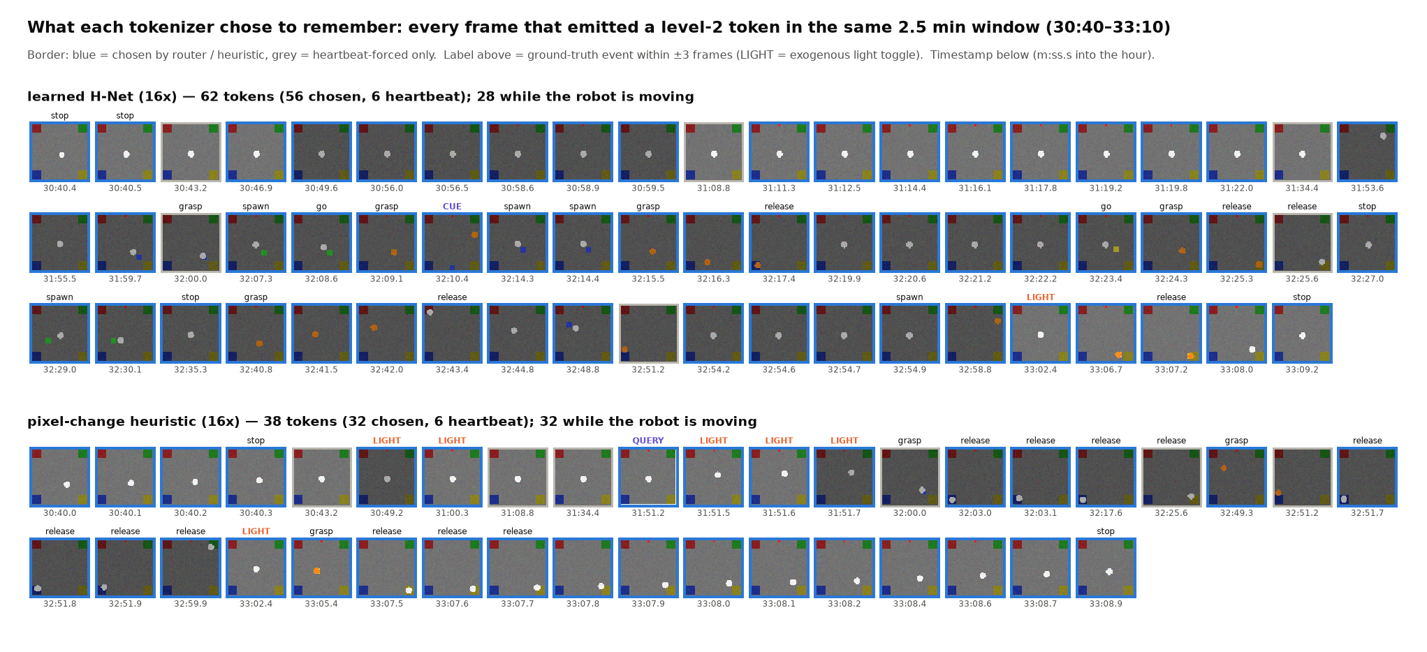
Figure 11. Every frame at which the learned model (top) and the pixel-change heuristic (bottom) emitted a level-2 token in the same 2.5-minute window, with timestamps and ground-truth events within ±3 frames.
7. Limitations
- Synthetic environment, toy scale. The environment is synthetic, low-resolution (64×64) and single-camera. Models are about 40M parameters with one vector per frame. The real-scale numbers in Figure 6 are projections from measured step latencies, not end-to-end measurements.
- Single seed. Each configuration was trained once (seed 0), for 4,000 steps. Differences of a few points in recall are within noise. The memory intervals in Figure 10 are wide.
- Not Mamba-2. Outer stages use sliding-window attention rather than H-Net’s Mamba-2. We do not expect this to change the conclusions, but it has not been tested.
- No spatial chunking. Spatial compression is a fixed CNN. Cartesia’s 2-D pixel-space H-Net has not been attempted.
- Toy-scale latency is launch-bound. No CUDA graphs or compiled kernels were used, so latency at this size does not reflect the FLOP gap between dense and event-driven models.
8. Next experiments
- Router. Tied or temperature-scaled cosine, or difference routing. Require a bimodal $p_t$ distribution and better-than-random event recall before reporting boundary results.
- Make memory pay. Predict action chunks (ACT-style) instead of single actions, remove $a_{t-1}$ from the policy input, and add a self-supervised retrieval loss that predicts properties of frames $k \in [64, 36{,}000]$ steps back. Then rerun the fixed / heuristic / learned comparison; that is where Cartesia’s ordering can actually appear.
- Sparse frame encoder. A patch-level change router (as in Eventful Transformers), or a 2-D H-Net stage 0, so that per-frame cost scales with changed pixels.
- One day of context. Add an L3 stage around the trained main network and train it on cached L2 outputs from day-long logs.
- Real data. Test whether learned boundaries coincide with contacts, failures and human interventions in real robot logs.
9. Conclusion
Learned, causal chunking turns long-context video from a memory problem into an event-rate problem. The streaming engine runs the expensive network only when a top-level token fires, matches the training-time model exactly, and makes a day of robot video fit on a single consumer GPU. Whether the learned part earns its name is still open. In our setting the router collapsed onto its threshold, and the objective never asked the model to remember. Both have concrete fixes, and the evaluation tools in this post (boundary recall against random, idle versus active cost, grouped probes) are what we will use to tell when they work.
图 11. 在同一个 2.5 分钟的窗口内,学习模型(上)和像素变化启发式(下)发出第二层 token 的每一帧,标注了时间戳和 ±3 帧内的事件真值。
7. 局限
- 合成环境、玩具规模。 环境是合成的、低分辨率(64×64)、单相机。模型约 4000 万参数,每帧一个向量。图 6 中的真实规模数字是根据实测单步延迟推算的,不是端到端的测量。
- 单个种子。 每个配置只训练了一次(种子 0),4,000 步。召回率相差几个百分点,属于噪声范围之内;图 10 中记忆的置信区间很宽。
- 不是 Mamba-2。 外层用的是滑动窗口注意力,而不是 H-Net 的 Mamba-2。我们预计这不会改变结论,但没有验证过。
- 没有空间分块。 空间压缩是一个固定的 CNN,Cartesia 的二维像素空间 H-Net 还没有尝试。
- 玩具规模下的延迟受限于 kernel 启动。 没有用 CUDA graphs 或编译过的 kernel,所以这个规模下的延迟反映不出稠密与事件驱动之间的 FLOPs 差距。
8. 下一步实验
- router。 绑定或带温度的余弦,或差分路由。在报告任何边界结果之前,要求 $p_t$ 分布呈双峰,且事件召回率优于随机。
- 让记忆有回报。 预测动作块(ACT 风格)而不是单步动作,从策略输入中去掉 $a_{t-1}$,并加一个自监督检索损失,预测 $k \in [64, 36{,}000]$ 步之前那一帧的属性。然后重跑固定 / 启发式 / 学习三者的对比;Cartesia 的那个排序,只有在这里才可能真正显现。
- 稀疏帧编码器。 patch 级别的变化 router(参照 Eventful Transformers),或者二维 H-Net 作为第 0 阶段,让每帧开销随变化的像素数伸缩。
- 一整天的上下文。 在训练好的主网络外面加一个 L3 阶段,用一整天日志的缓存 L2 输出来训练。
- 真实数据。 检验学出来的边界是否与真实机器人日志中的接触、失败和人工干预重合。
9. 结论
学习式的因果分块,把长上下文视频从一个显存问题变成了一个事件速率问题。流式引擎只在顶层 token 触发时才运行昂贵的网络,与训练时的模型完全一致,让一整天的机器人视频能放进一张消费级 GPU。至于学习这一部分是否名副其实,还是开放问题:在我们的设定里,router 塌缩到了阈值上,目标函数也从未要求模型去记忆。两者都有具体的修法,而这篇文章里的评测工具(与随机边界对比的事件召回、空闲与活跃的开销对比、分组探针),就是我们用来判断它们何时奏效的标准。
References
- Tokens to bytes: Cartesia, From Tokens to Bytes, part 1 and part 2
- H-Net: Hwang, Wang, Gu, Dynamic Chunking for End-to-End Hierarchical Sequence Modeling (arXiv:2507.07955)
- BLT: Pagnoni et al., Byte Latent Transformer: Patches Scale Better Than Tokens (arXiv:2412.09871)
- Mamba-2: Dao & Gu, Transformers are SSMs (arXiv:2405.21060)
- Copycat in behaviour cloning: Wen et al., Fighting Copycat Agents in Behavioral Cloning from Observation Histories (arXiv:2010.14876)
- Action chunking: Zhao et al., Learning Fine-Grained Bimanual Manipulation with Low-Cost Hardware (ACT) (arXiv:2304.13705)
- Sparse per-frame compute: Dutson et al., Eventful Transformers (arXiv:2308.13494)
参考文献
- 从 token 到字节 — Cartesia,From Tokens to Bytes,第一篇、第二篇
- H-Net — Hwang, Wang, Gu,Dynamic Chunking for End-to-End Hierarchical Sequence Modeling(arXiv:2507.07955)
- BLT — Pagnoni 等,Byte Latent Transformer: Patches Scale Better Than Tokens(arXiv:2412.09871)
- Mamba-2 — Dao & Gu,Transformers are SSMs(arXiv:2405.21060)
- 行为克隆中的 copycat — Wen 等,Fighting Copycat Agents in Behavioral Cloning from Observation Histories(arXiv:2010.14876)
- 动作分块 — Zhao 等,Learning Fine-Grained Bimanual Manipulation with Low-Cost Hardware(ACT)(arXiv:2304.13705)
- 逐帧稀疏计算 — Dutson 等,Eventful Transformers(arXiv:2308.13494)